3.6 Associative Models/ Causal (Econometric) Forecasting
Associative model forecasting methods, also known as causal or econometric forecasting methods, are quantitative techniques used in operations management to predict future values of a variable by analyzing its relationship with other related variables. These methods are particularly useful when historical data is available for both the variable of interest and the potential causal factors influencing it.
Associative forecasting models, unlike time-series methods, consider multiple independent variables (causal factors) that are related to or influence the forecasted dependent variable. These models aim to establish and quantify the cause-and-effect relationships between the independent and dependent variables, enabling more accurate predictions by accounting for the impact of various factors. These factors, termed explanatory variables, can significantly improve the accuracy of forecasts. For instance, incorporating climate data into a sales forecast model for umbrellas can enhance its predictive power.
Some forecasting methods try to identify the underlying factors that might influence the variable being forecasted. For example, including information about climate patterns might improve the ability of a model to predict umbrella sales. Forecasting models often take account of regular seasonal variations. In addition to climate, such variations can also be due to holidays and customs: for example, one might predict that sales of college football apparel will be higher during the football season than during the off-season.
Regression Analysis
Regression analysis is one of the most widely used associative forecasting methods, which involves constructing a mathematical equation that relates the dependent variable to one or more independent variables. This statistical technique estimates the relationships between variables. It encompasses a diverse set of methods for modelling and analyzing the interplay between a dependent variable (the variable being forecast) and one or more independent variables (factors believed to influence the dependent variable). Regression analysis is particularly valuable for understanding how changes in independent variables impact the average value of the dependent variable while holding all other independent variables constant.
The coefficients of the independent variables in the regression equation represent the magnitude and direction of their impact on the dependent variable.
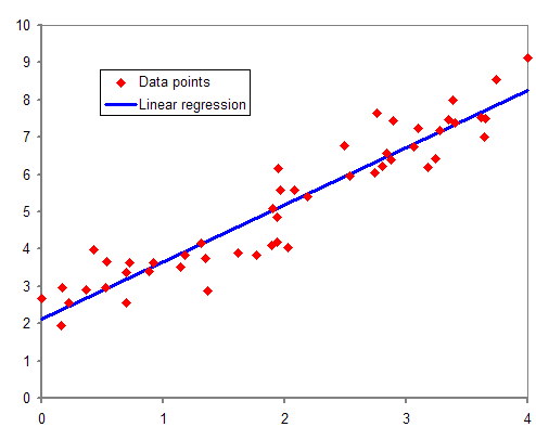
Image Description
The image is a scatter plot depicting data points and a linear regression line. The x-axis ranges from 0 to 4. The y-axis ranges from 0 to 10. The red diamonds represent the data points. The blue line represents the linear regression line, showing the best-fit line through the data points.
The data points follow an upward trend, indicating a positive correlation between the variables. The linear regression line slopes upward from left to right, suggesting a strong linear relationship. The legend in the plot identifies the red diamonds as “Data points” and the blue line as “Linear regression.”
Simple Linear Regression
In its simplest form, a linear regression model with a single independent variable can be expressed as:
Y = bX + a
Where:
‘Y’ is the dependent variable (the variable being forecasted)
‘X’ is the independent variable (the causal factor)
‘b’ is a slope of the regression line (a measure of its steepness, i.e. the ratio of the rise to the run, or rise divided by the run)
‘a’ is Y-intercept (the point on the Y-axis by which the slope of the line sweeps)
Multiple Linear Regression
When there are multiple independent variables influencing the dependent variable, a multiple linear regression model can be employed:
Y = a + b₁X₁ + b₂X₂ + … + bₙXₙ
Where:
- X₁, X₂, …, Xₙ are the independent variables (causal factors)
- b₁, b₂, …, bₙ are the regression coefficients associated with each independent variable
Correlation Analysis
Correlation analysis is often used with regression analysis to measure the strength and direction of the linear relationship between the dependent and independent variables. The correlation coefficient, denoted by r, ranges from -1 to 1, with values closer to 1 or -1 indicating a stronger linear relationship and values closer to 0 indicating a weaker or no linear relationship.
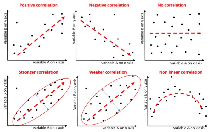
Figure 3.6.2 consists of six scatter plot diagrams demonstrating correlations between variables A (on the x-axis) and B (on the y-axis).
- Positive correlation: A scatter plot with points roughly following an upward-sloping line from the bottom left to the top right. The red dashed line indicates a positive slope.
- Negative correlation: A scatter plot with points roughly following a downward-sloping line from the top left to the bottom right. The red dashed line indicates a negative slope.
- No correlation: A scatter plot with points scattered randomly with no discernible pattern. The red dashed line is flat, indicating no correlation.
- Stronger correlation: A scatter plot where points are tightly clustered around a red dashed upward-sloping line. The points are enclosed within a narrow ellipse.
- Weaker correlation: A scatter plot where points are more loosely clustered around a red dashed upward-sloping line. The points are enclosed within a wider ellipse.
- Non-linear correlation: A scatter plot where points follow a curved pattern, suggesting a quadratic relationship. The red dashed line forms an upward arch, indicating a non-linear correlation.
Applications in Operations Management
Associative forecasting methods are widely used in operations management for various purposes, including:
- Demand forecasting: Predicting future demand for products or services by considering advertising expenditure, competitor pricing, economic indicators, and demographic variables.
- Capacity planning: Estimating the required production capacity by analyzing the relationships between demand, production rates, and other operational factors.
- Inventory management: Forecasting inventory levels by considering factors such as demand patterns, lead times, and supply chain dynamics.
- Resource allocation: Optimizing the allocation of resources (e.g., workforce, materials, equipment) based on forecasted demand and operational constraints.
- Supply chain management: Predicting supply chain performance metrics (e.g., lead times, costs, service levels) by considering factors such as supplier performance, transportation modes, and logistics networks.
(Frenzel, 2023).
Associative forecasting methods provide a powerful tool for operations managers to make informed decisions by accounting for the complex relationships between various factors and the variables of interest. However, it is crucial to ensure the validity of the underlying assumptions, the quality of the data, and the appropriate selection and evaluation of the forecasting models.
Common Forecasting Assumptions
- Forecasts are rarely, if ever, perfect. It is nearly impossible to estimate 100% accurately what the future will hold. Firms need to understand and expect some errors in their forecasts.
- Forecasts tend to be more accurate for groups of items than for individual items in the group. The popular Fitbit may be producing six different models. Each model may be offered in several different colours. Each of those colours may come in small, large, and extra large. The forecast for each model will be far more accurate than the forecast for each specific end item.
- Forecast accuracy will tend to decrease as the time horizon increases. The farther away the forecast is from the current date, the more uncertainty it will contain.
“3 Forecasting” from Introduction to Operations Management Copyright © by Hamid Faramarzi and Mary Drane is licensed under a Creative Commons Attribution-NonCommercial-ShareAlike 4.0 International License, except where otherwise noted. Modifications: expanded content and added new content on Linear Regression, Correlation Analysis, & Applications in Operations Management.
