5.3 Centripetal Force
Learning Objectives
By the end of this section, you will be able to:
- Calculate coefficient of friction on a car tire.
- Calculate ideal speed and angle of a car on a turn.
Any force or combination of forces can cause a centripetal or radial acceleration. Just a few examples are the tension in the rope on a tether ball, the force of Earth’s gravity on the Moon, friction between roller skates and a rink floor, a banked roadway’s force on a car, and forces on the tube of a spinning centrifuge.
Any net force causing uniform circular motion is called a centripetal force. The direction of a centripetal force is toward the center of curvature, the same as the direction of centripetal acceleration. According to Newton’s second law of motion, net force is mass times acceleration: net [latex]\text{F} = \text{ma}[/latex]. For uniform circular motion, the acceleration is the centripetal acceleration— [latex]a = a_{c}[/latex]. Thus, the magnitude of centripetal force [latex]\text{F}_{\text{c}}[/latex] is
[latex]\text{F}_{\text{c}} = \left(m \text{a}\right)_{\text{c}} .[/latex]
By using the expressions for centripetal acceleration [latex]a_{c}[/latex] from [latex]a_{c} = \frac{v^{2}}{r} ; a_{c} = rω^{2}[/latex], we get two expressions for the centripetal force [latex]\text{F}_{\text{c}}[/latex] in terms of mass, velocity, angular velocity, and radius of curvature:
[latex]F_{c} = m \frac{v^{2}}{r} ; F_{c} = \text{mr} \omega^{2} .[/latex]
You may use whichever expression for centripetal force is more convenient. Centripetal force [latex]F_{\text{c}}[/latex] is always perpendicular to the path and pointing to the center of curvature, because [latex]\mathbf{a}_{c}[/latex] is perpendicular to the velocity and pointing to the center of curvature.
Note that if you solve the first expression for [latex]r[/latex], you get
[latex]r = \frac{mv^{2}}{F_{c}} .[/latex]
This implies that for a given mass and velocity, a large centripetal force causes a small radius of curvature—that is, a tight curve.
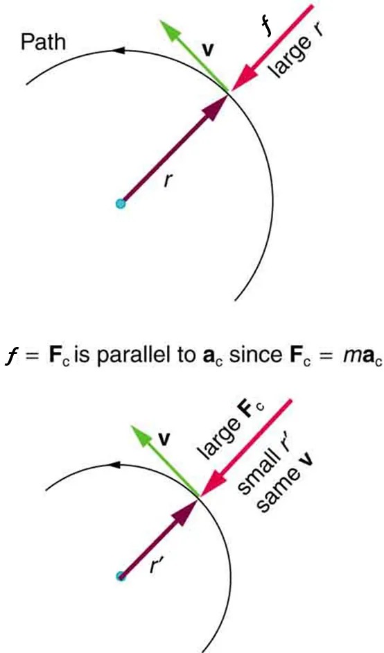
Figure 5.9 The frictional force supplies the centripetal force and is numerically equal to it. Centripetal force is perpendicular to velocity and causes uniform circular motion. The larger the [latex]\text{F}_{\text{c}}[/latex], the smaller the radius of curvature [latex]r[/latex] and the sharper the curve. The second curve has the same [latex]v[/latex], but a larger [latex]\text{F}_{\text{c}}[/latex] produces a smaller [latex]r '[/latex]. Image from OpenStax College Physics 2e, CC-BY 4.0
Image Description
The image consists of two diagrams illustrating centripetal force in circular motion.
Top Diagram:
– A circle is depicted, with a point on its circumference.
– A vector labeled “v” is shown in green, pointing tangentially to the circle, indicating velocity.
– A vector labeled “f” is shown in red, pointing radially inward towards the circle’s center, indicating force.
– A vector labeled “r” is pointing from the circle’s center to the point on its circumference.
– Text labels this situation as “large r.”
Bottom Diagram:
– Another circle, with a smaller radius than the first, is depicted with a point on its circumference.
– A green vector labeled “v” points tangentially to the circle, indicating velocity, with the note “same v.”
– A red vector labeled “large Fc” points radially inward, indicating a larger centripetal force compared to the first diagram.
– A vector labeled “r'” points from the circle’s center to the point on its circumference.
– Text labels this as “small r’.”
Additional Text:
– Between the diagrams, there is an explanation: “f = Fc is parallel to ac since Fc = mac”, indicating the relationship between centripetal force and acceleration.
Example 5.4
What Coefficient of Friction Do Car Tires Need on a Flat Curve?
(a) Calculate the centripetal force exerted on a 900 kg car that negotiates a 500 m radius curve at 25.0 m/s.
(b) Assuming an unbanked curve, find the minimum static coefficient of friction, between the tires and the road, static friction being the reason that keeps the car from slipping (see Figure 5.10).
Strategy and Solution for (a)
We know that [latex]F_{\text{c}} = \frac{mv^{\text{2}}}{r}[/latex]. Thus,
[latex]F_{\text{c}} = \frac{mv^{\text{2}}}{r} = \frac{\left(\right. \text{900 kg} \left.\right) \left(\right. \text{25}.\text{0 m}/\text{s} \left.\right)^{\text{2}}}{\left(\right. \text{500 m} \left.\right)} = \text{1125 N}.[/latex]
Strategy for (b)
Figure 5.10 shows the forces acting on the car on an unbanked (level ground) curve. Friction is to the left, keeping the car from slipping, and because it is the only horizontal force acting on the car, the friction is the centripetal force in this case. We know that the maximum static friction (at which the tires roll but do not slip) is [latex]\mu_{\text{s}} N[/latex], where [latex]\mu_{\text{s}}[/latex] is the static coefficient of friction and N is the normal force. The normal force equals the car’s weight on level ground, so that
[latex]N = \mathit{mg}[/latex]. Thus the centripetal force in this situation is
[latex]F_{\text{c}} = f = \mu_{\text{s}} N = \mu_{\text{s}} \text{mg} .[/latex]
Now we have a relationship between centripetal force and the coefficient of friction. Using the first expression for [latex]F_{\text{c}}[/latex] from the equation
[latex]\left.\begin{align*} F_{\text{c}} &= m \frac{v^{2}}{r} \\[1.5ex] F_{\text{c}} &= \text{mr} \omega^{2}\end{align*}\right\},[/latex]
[latex]m \frac{v^{2}}{r} = \mu_{\text{s}} \text{mg} .[/latex]
We solve this for [latex]\mu_{\text{s}}[/latex], noting that mass cancels, and obtain
[latex]\mu_{\text{s}} = \frac{v^{2}}{\text{rg}} .[/latex]
Solution for (b)
Substituting the knowns,
[latex]\mu_{\text{s}} = \frac{\left(\right. \text{25}.\text{0 m}/\text{s} \left.\right)^{2}}{\left(\right. \text{500 m} \left.\right) \left(\right. 9 . \text{80 m}/\text{s}^{2} \left.\right)} = 0 . \text{13} .[/latex]
(Because coefficients of friction are approximate, the answer is given to only two digits.)
Discussion
We could also solve part (a) using the first expression in [latex]\left.\begin{align*}F_{\text{c}} &= m \frac{v^{2}}{r} \\ F_{\text{c}} &= \text{mr} \omega^{2}\end{align*} \right\} ,[/latex] because [latex]m ,[/latex][latex]v ,[/latex] and [latex]r[/latex] are given. The coefficient of friction found in part (b) is much smaller than is typically found between tires and roads. The car will still negotiate the curve if the coefficient is greater than 0.13, because static friction is a responsive force, being able to assume a value less than but no more than [latex]\mu_{\text{s}} N[/latex]. A higher coefficient would also allow the car to negotiate the curve at a higher speed, but if the coefficient of friction is less, the safe speed would be less than 25 m/s. Note that mass cancels, implying that in this example, it does not matter how heavily loaded the car is to negotiate the turn. Mass cancels because friction is assumed proportional to the normal force, which in turn is proportional to mass. If the surface of the road were banked, the normal force would be less as will be discussed below.
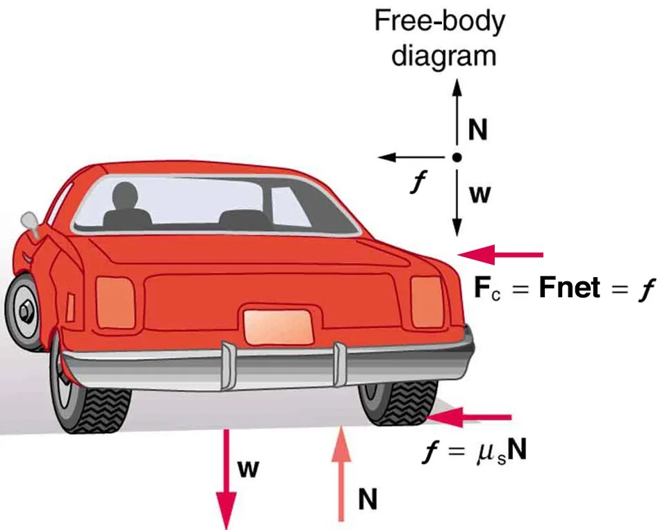
Figure 5.10 This car on level ground is moving away and turning to the left. The centripetal force causing the car to turn in a circular path is due to friction between the tires and the road. A minimum coefficient of friction is needed, or the car will move in a larger-radius curve and leave the roadway. Image from OpenStax College Physics 2e, CC-BY 4.0
Image Description
The image depicts a red car viewed from the rear. Alongside the car, there is a free-body diagram illustrating the various forces acting on it.
– Forces and Labels:
– An upward arrow labeled “N” represents the normal force.
– A downward arrow labeled “w” indicates the weight of the car.
– A leftward arrow labeled “f” represents friction.
– To the right of the car, the equation “Fc = Fnet = f” is noted, highlighting the net force.
– Another notation in the lower right explains “f = μsN”, where “μs” is the coefficient of static friction and “N” is the normal force.
– Additional Details:
– The car has a visible rear bumper, taillights, and tires.
– There is a side mirror on the car’s left side.
– The car appears to be on a flat surface.
The diagram serves to illustrate the physics of forces involved, particularly focusing on friction, weight, and normal force.
Let us now consider banked curves, where the slope of the road helps you negotiate the curve. See Figure 5.11. The greater the angle [latex]\theta[/latex], the faster you can take the curve. Race tracks for bikes as well as cars, for example, often have steeply banked curves. In an “ideally banked curve,” the angle [latex]\theta[/latex] is such that you can negotiate the curve at a certain speed without the aid of friction between the tires and the road. We will derive an expression for [latex]\theta[/latex] for an ideally banked curve and consider an example related to it.
For ideal banking, the net external force equals the horizontal centripetal force in the absence of friction. The components of the normal force N in the horizontal and vertical directions must equal the centripetal force and the weight of the car, respectively. In cases in which forces are not parallel, it is most convenient to consider components along perpendicular axes—in this case, the vertical and horizontal directions.
Figure 5.11 shows a free body diagram for a car on a frictionless banked curve. If the angle [latex]\theta[/latex] is ideal for the speed and radius, then the net external force will equal the necessary centripetal force. The only two external forces acting on the car are its weight [latex]\mathbf{w}[/latex] and the normal force of the road [latex]\mathbf{N}[/latex]. (A frictionless surface can only exert a force perpendicular to the surface—that is, a normal force.) These two forces must add to give a net external force that is horizontal toward the center of curvature and has magnitude [latex]\text{mv}^{2} /\text{r}[/latex]. Because this is the crucial force and it is horizontal, we use a coordinate system with vertical and horizontal axes. Only the normal force has a horizontal component, and so this must equal the centripetal force—that is,
[latex]N \text{sin} \theta = \frac{mv^{2}}{r} .[/latex]
Because the car does not leave the surface of the road, the net vertical force must be zero, meaning that the vertical components of the two external forces must be equal in magnitude and opposite in direction. From the figure, we see that the vertical component of the normal force is [latex]N \text{cos} \theta[/latex], and the only other vertical force is the car’s weight. These must be equal in magnitude; thus,
[latex]N \text{cos} \theta = \text{mg} .[/latex]
Now we can combine the last two equations to eliminate [latex]N[/latex] and get an expression for [latex]\theta[/latex], as desired. Solving the second equation for [latex]N = \text{mg} / \left(\right. \text{cos} \theta \left.\right)[/latex], and substituting this into the first yields
[latex]\text{mg} \frac{\text{sin} \theta}{\text{cos} \theta} = \frac{\text{mv}^{2}}{r}[/latex]
[latex]\begin{eqnarray*}\text{mg} \text{tan} \left(\right. \theta \left.\right) & = & \frac{mv^{2}}{r} \\ \text{tan} \theta & = & \frac{v^{2}}{\text{rg}.}\end{eqnarray*}[/latex]
Taking the inverse tangent gives
[latex]\theta = \text{tan}^{- 1} \left(\frac{v^{2}}{\text{rg}}\right) \text{ }(\text{ideally banked curve},\text{ no friction}).[/latex]
This expression can be understood by considering how [latex]\theta[/latex] depends on [latex]v[/latex] and [latex]r[/latex]. A large [latex]\theta[/latex] will be obtained for a large [latex]v[/latex] and a small [latex]r[/latex]. That is, roads must be steeply banked for high speeds and sharp curves. Friction helps, because it allows you to take the curve at greater or lower speed than if the curve is frictionless. Note that [latex]\theta[/latex] does not depend on the mass of the vehicle.
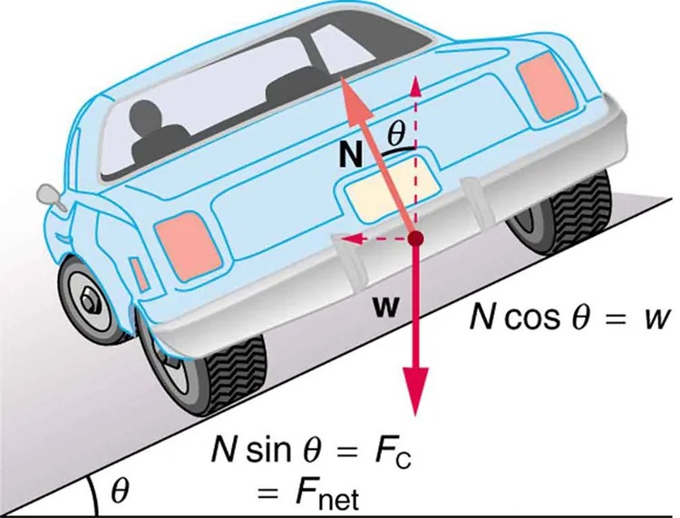
Figure 5.11 The car on this banked curve is moving away and turning to the left. Image from OpenStax College Physics 2e, CC-BY 4.0
Image Description
The image shows a blue car positioned on an inclined surface. The car is viewed slightly from the rear and side, with two visible passengers inside. The rear left tire is clearly visible, as the car is tilted downward along the slope.
Several vector arrows and mathematical notations are overlaid on the image to depict forces acting on the car:
- A red dashed arrow labeled N extends vertically upward from the center of the car, and a red solid arrow labeled w points downward, indicating the weight.
- An angular notation θ is shown where the vertical dashed line of N extends from the car, depicting the angle between the normal force and the inclined plane.
- A horizontal red arrow is directed to the left, labeled with equations: N sin θ = Fc = Fnet, showing the component of force parallel to the incline.
- Two other equations are included: N cos θ = w, showing the perpendicular component of the weight, in line with the normal force.
- An arc labeled θ is shown at the bottom left, representing the incline’s angle relative to the horizontal.
The diagram illustrates the forces and components acting on a car on an inclined plane, focusing on the normal force and weight relationship.
Example 5.5
What Is the Ideal Speed to Take a Steeply Banked Tight Curve?
Curves on some test tracks and race courses, such as the Daytona International Speedway in Florida, are very steeply banked. This banking, with the aid of tire friction and very stable car configurations, allows the curves to be taken at very high speed. To illustrate, calculate the speed at which a 100 m radius curve banked at 65.0° should be driven if the road is frictionless.
Strategy
We first note that all terms in the expression for the ideal angle of a banked curve except for speed are known; thus, we need only rearrange it so that speed appears on the left-hand side and then substitute known quantities.
Solution
Starting with
[latex]\text{tan} \theta = \frac{v^{2}}{\text{rg}}[/latex]
we get
[latex]v = \left(\right. \text{rg} \text{tan} \theta \left.\right)^{1 / 2} .[/latex]
Noting that tan 65.0º = 2.14, we obtain
[latex]\begin{eqnarray*}v & = & \left[\left(\right. \text{100 m} \left.\right) \left(\right. 9.80 m /\text{s}^{2} \left.\right) \left(\right. 2 . \text{14} \left.\right)\right]^{1 / 2} \\ & = & \text{45}.\text{8 m}/\text{s}.\end{eqnarray*}[/latex]
Discussion
This is just about 165 km/h, consistent with a very steeply banked and rather sharp curve. Tire friction enables a vehicle to take the curve at significantly higher speeds.
Calculations similar to those in the preceding examples can be performed for a host of interesting situations in which centripetal force is involved—a number of these are presented in this chapter’s Problems and Exercises.
Take-Home Experiment
Ask a friend or relative to swing a golf club or a tennis racquet. Take appropriate measurements to estimate the centripetal acceleration of the end of the club or racquet. You may choose to do this in slow motion.
PhET Explorations
Gravity and Orbits
Move the sun, earth, moon and space station to see how it affects their gravitational forces and orbital paths. Visualize the sizes and distances between different heavenly bodies, and turn off gravity to see what would happen without it!
