4.9 Friction
Learning Objectives
By the end of this section, you will be able to:
- Discuss the general characteristics of friction.
- Describe the various types of friction.
- Calculate the magnitude of static and kinetic friction.
Friction is a force that is around us all the time that opposes relative motion between surfaces in contact but also allows us to move (which you have discovered if you have ever tried to walk on ice). While a common force, the behavior of friction is actually very complicated and is still not completely understood. We have to rely heavily on observations for whatever understandings we can gain. However, we can still deal with its more elementary general characteristics and understand the circumstances in which it behaves.
Friction
Friction is a force that opposes relative motion between surfaces in contact.
One of the simpler characteristics of friction is that it is parallel to the contact surface between surfaces and always in a direction that opposes motion or attempted motion of the systems relative to each other. If two surfaces are in contact and moving relative to one another, then the friction between them is called kinetic friction. For example, friction slows a hockey puck sliding on ice. But when objects are stationary, static friction can act between them; the static friction is usually greater than the kinetic friction between the surfaces.
Kinetic Friction
If two surfaces are in contact and moving relative to one another, then the friction between them is called kinetic friction.
Imagine, for example, trying to slide a heavy crate across a concrete floor—you may push harder and harder on the crate and not move it at all. This means that the static friction responds to what you do—it increases to be equal to and in the opposite direction of your push. But if you finally push hard enough, the crate seems to slip suddenly and starts to move. Once in motion it is easier to keep it in motion than it was to get it started, indicating that the kinetic friction force is less than the static friction force. If you add mass to the crate, say by placing a box on top of it, you need to push even harder to get it started and also to keep it moving. Furthermore, if you oiled the concrete you would find it to be easier to get the crate started and keep it going (as you might expect).
Figure 4.29 is a crude pictorial representation of how friction occurs at the interface between two objects. Close-up inspection of these surfaces shows them to be rough. So when you push to get an object moving (in this case, a crate), you must raise the object until it can skip along with just the tips of the surface hitting, break off the points, or do both. A considerable force can be resisted by friction with no apparent motion. The harder the surfaces are pushed together (such as if another box is placed on the crate), the more force is needed to move them. Part of the friction is due to adhesive forces between the surface molecules of the two objects, which explain the dependence of friction on the nature of the substances. Adhesion varies with substances in contact and is a complicated aspect of surface physics. Once an object is moving, there are fewer points of contact (fewer molecules adhering), so less force is required to keep the object moving. At small but nonzero speeds, friction is nearly independent of speed.
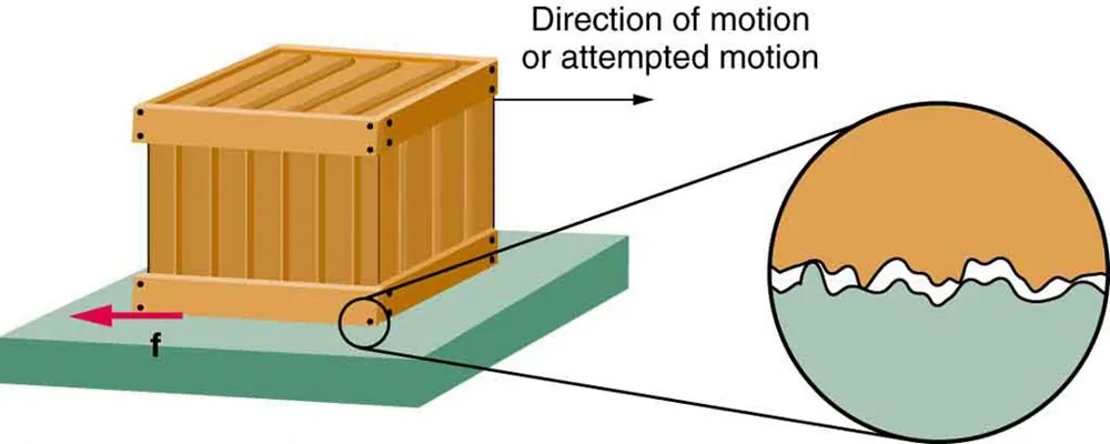
Figure 4.29 Frictional forces, such as [latex]f[/latex], always oppose motion or attempted motion between surfaces in contact. Friction arises in part because of the roughness of the surfaces in contact, as seen in the expanded view. In order for the object to move, it must rise to where the peaks can skip along the bottom surface. Thus a force is required just to set the object in motion. Some of the peaks will be broken off, also requiring a force to maintain motion. Much of the friction is actually due to attractive forces between molecules making up the two objects, so that even perfectly smooth surfaces are not friction-free. Such adhesive forces also depend on the substances the surfaces are made of, explaining, for example, why rubber-soled shoes slip less than those with leather soles. Image from OpenStax College Physics 2e, CC-BY 4.0
Image Description
The image shows a diagram illustrating the concept of friction. There is a rectangular wooden crate resting on a flat, green surface. An arrow labeled “Direction of motion or attempted motion” points to the right, indicating the intended or actual movement of the crate. Another arrow labeled “f” points to the left, representing the force of friction opposing the motion.
On the right side of the image, there is an enlarged circular view that zooms in on the contact area between the crate and the surface. This close-up shows a rough, uneven interaction between the surfaces, highlighting the microscopic irregularities that contribute to friction.
The diagram helps to explain how friction works by showing both the direction of the applied force and the opposing frictional force, as well as the surface roughness involved.
The magnitude of the frictional force has two forms: one for static situations (static friction), the other for when there is motion (kinetic friction).
When there is no motion between the objects, the magnitude of static friction [latex]\mathbf{f}_{\text{s}}[/latex] is
[latex]f_{s} \leq \mu_{s} N ,[/latex]
where [latex]\mu_{\text{s}}[/latex] is the coefficient of static friction and [latex]N[/latex] is the magnitude of the normal force (the force perpendicular to the surface).
Magnitude of Static Friction
Magnitude of static friction [latex]f_{\text{s}}[/latex] is
[latex]f_{\text{s}} \leq \mu_{\text{s}} N ,[/latex]
where [latex]\mu_{\text{s}}[/latex] is the coefficient of static friction and [latex]N[/latex] is the magnitude of the normal force.
The symbol [latex]\leq[/latex] means less than or equal to, implying that static friction can have a minimum and a maximum value of [latex]\mu_{\text{s}} N[/latex]. Static friction is a responsive force that increases to be equal and opposite to whatever force is exerted, up to its maximum limit. Once the applied force exceeds [latex]f_{\text{s} \left(\right. \text{max} \left.\right)}[/latex], the object will move. Thus
[latex]f_{\text{s} \left(\right. \text{max} \left.\right)} = \mu_{\text{s}} N .[/latex]
Once an object is moving, the magnitude of kinetic friction [latex]\mathbf{f}_{\text{k}}[/latex] is given by
[latex]f_{\text{k}} = \mu_{\text{k}} N ,[/latex]
where [latex]\mu_{\text{k}}[/latex] is the coefficient of kinetic friction. A system in which [latex]f_{\text{k}} = \mu_{\text{k}} N[/latex]is described as a system in which friction behaves simply.
Magnitude of Kinetic Friction
The magnitude of kinetic friction [latex]f_{\text{k}}[/latex] is given by
[latex]f_{\text{k}} = \mu_{\text{k}} N ,[/latex]
where [latex]\mu_{\text{k}}[/latex] is the coefficient of kinetic friction.
As seen in Table 4.2, the coefficients of kinetic friction are less than their static counterparts. That values of [latex]\mu[/latex] in Table 4.2 are stated to only one or, at most, two digits is an indication of the approximate description of friction given by the above two equations.
| System | Static friction[latex]\mu_{\text{s}}[/latex] | Kinetic friction[latex]\mu_{\text{k}}[/latex] |
|---|---|---|
| Rubber on dry concrete | 1.0 | 0.7 |
| Rubber on wet concrete | 0.7 | 0.5 |
| Wood on wood | 0.5 | 0.3 |
| Waxed wood on wet snow | 0.14 | 0.1 |
| Metal on wood | 0.5 | 0.3 |
| Steel on steel (dry) | 0.6 | 0.3 |
| Steel on steel (oiled) | 0.05 | 0.03 |
| Teflon on steel | 0.04 | 0.04 |
| Bone lubricated by synovial fluid | 0.016 | 0.015 |
| Shoes on wood | 0.9 | 0.7 |
| Shoes on ice | 0.1 | 0.05 |
| Ice on ice | 0.1 | 0.03 |
| Steel on ice | 0.04 | 0.02 |
Table 4.2
Coefficients of Static and Kinetic FrictionThe equations given earlier include the dependence of friction on materials and the normal force. The direction of friction is always opposite that of motion, parallel to the surface between objects, and perpendicular to the normal force. For example, if the crate you try to push (with a force parallel to the floor) has a mass of 100 kg, then the normal force would be equal to its weight, [latex]W = mg = \left(\right. \text{100 kg} \left.\right) \left(\right. 9 . \text{80} \text{m}/\text{s}^{2} \left.\right) = \text{980 N}[/latex], perpendicular to the floor. If the coefficient of static friction is 0.45, you would have to exert a force parallel to the floor greater than
[latex]f_{\text{s} \left(\right. \text{max} \left.\right)} = \mu_{\text{s}} N = \left(0.45\right) \left(\right. \text{980} \text{N} \left.\right) = \text{440} \text{N}[/latex]to move the crate. Once there is motion, friction is less and the coefficient of kinetic friction might be 0.30, so that a force of only 290 N
([latex]f_{\text{k}} = \mu_{\text{k}} N = \left(0 . \text{30}\right) \left(\text{980} \text{N}\right) = \text{290} \text{N}[/latex])
would keep it moving at a constant speed. If the floor is lubricated, both coefficients are considerably less than they would be without lubrication. Coefficient of friction is a unitless quantity with a magnitude usually between 0 and 1.0. The coefficient of the friction depends on the two surfaces that are in contact.
Take-Home Experiment
Find a small plastic object (such as a food container) and slide it on a kitchen table by giving it a gentle tap. Now spray water on the table, simulating a light shower of rain. What happens now when you give the object the same-sized tap? Now add a few drops of (vegetable or olive) oil on the surface of the water and give the same tap. What happens now? This latter situation is particularly important for drivers to note, especially after a light rain shower. Why?
Many people have experienced the slipperiness of walking on ice. However, many parts of the body, especially the joints, have much smaller coefficients of friction—often three or four times less than ice. A joint is formed by the ends of two bones, which are connected by thick tissues. The knee joint is formed by the lower leg bone (the tibia) and the thighbone (the femur). The hip is a ball (at the end of the femur) and socket (part of the pelvis) joint. The ends of the bones in the joint are covered by cartilage, which provides a smooth, almost glassy surface. The joints also produce a fluid (synovial fluid) that reduces friction and wear. A damaged or arthritic joint can be replaced by an artificial joint (Figure 4.30). These replacements can be made of metals (stainless steel or titanium) or plastic (polyethylene), also with very small coefficients of friction.
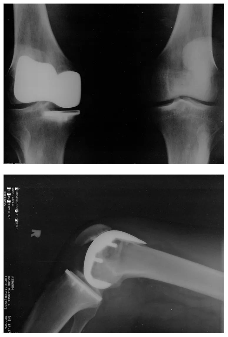
Figure 4.30 Artificial knee replacement is a procedure that has been performed for more than 20 years. In this figure, we see the post-op X-rays of the right knee joint replacement. Image from OpenStax College Physics 2e, CC-BY 4.0
Other natural lubricants include saliva produced in our mouths to aid in the swallowing process, and the slippery mucus found between organs in the body, allowing them to move freely past each other during heartbeats, during breathing, and when a person moves. Artificial lubricants are also common in hospitals and doctor’s clinics. For example, when ultrasonic imaging is carried out, the gel that couples the transducer to the skin also serves to lubricate the surface between the transducer and the skin—thereby reducing the coefficient of friction between the two surfaces. This allows the transducer to move freely over the skin.
Example 4.11
Skiing Exercise
A skier with a mass of 62 kg is sliding down a snowy slope. Find the coefficient of kinetic friction for the skier if friction is known to be 45.0 N.
Strategy
The magnitude of kinetic friction was given in to be 45.0 N. Kinetic friction is related to the normal force
[latex]N[/latex] as [latex]f_{\text{k}} = \mu_{\text{k}} N[/latex]; thus, the coefficient of kinetic friction can be found if we can find the normal force of the skier on a slope. The normal force is always perpendicular to the surface, and since there is no motion perpendicular to the surface, the normal force should equal the component of the skier’s weight perpendicular to the slope. (See the skier and free-body diagram in Figure 4.32.)
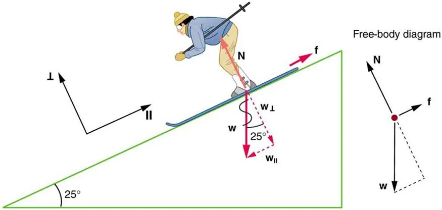
Figure 4.32 The motion of the skier and friction are parallel to the slope and so it is most convenient to project all forces onto a coordinate system where one axis is parallel to the slope and the other is perpendicular (axes shown to left of skier). [latex]\textbf{N}[/latex] (the normal force) is perpendicular to the slope, and [latex]\textbf{f}[/latex] (the friction) is parallel to the slope, but [latex]\textbf{w}[/latex] (the skier’s weight) has components along both axes, namely [latex]\textbf{w}_{⊥}[/latex] and [latex]\textbf{W}_{//}[/latex]. [latex]N[/latex] is equal in magnitude to [latex]w_{\bot}[/latex], so there is no motion perpendicular to the slope. However, [latex]f[/latex] is less than[latex]W_{//}[/latex] in magnitude, so there is acceleration down the slope Image from OpenStax College Physics 2e, CC-BY 4.0
Image Description
The image depicts a skier on a slope inclined at 25 degrees, along with a free-body diagram illustrating the forces acting on the skier.
– Skier Illustration:
– The skier is leaning forward, using ski poles for stability, and is positioned on skis sliding down the slope.
– The slope is represented by a green line inclined at an angle of 25 degrees.
– Forces on the Skier:
– N: The normal force is shown perpendicular to the slope, indicated by an arrow labeled “N.”
– f: The frictional force is depicted as an arrow pointing uphill along the slope, labeled “f.”
– w (Weight): The weight of the skier is directed vertically downward, labeled as “w.”
– The weight is decomposed into two components:
– w⊥: Perpendicular component of weight, directed into the slope.
– w‖: Parallel component of weight, directed down the slope.
– **Axes**:
– There are two sets of axes marked on the image:
– ⊥: Perpendicular to the slope.
– ‖: Parallel to the slope.
– Free-Body Diagram:
– Located to the right of the main skier illustration.
– It shows the same forces, with arrows indicating:
– Normal force (N) directed outwards and perpendicular.
– Frictional force (f) directed uphill.
– Weight (w) directed vertically downward.
– The diagram includes dashed lines denoting the components of the weight.
This setup illustrates the dynamics of the skier as they move down an inclined plane, emphasizing the interplay of gravitational, normal, and frictional forces.
That is,
[latex]N = w_{\bot} = w \text{cos} \text{25}º = \text{mg} \text{cos} \text{25}º .[/latex]
Substituting this into our expression for kinetic friction, we get
[latex]f_{\text{k}} = \mu_{\text{k}} \text{mg} \text{cos} \text{25}º ,[/latex]
which can now be solved for the coefficient of kinetic friction [latex]\mu_{\text{k}}[/latex].
Solution
Solving for [latex]\mu_{k}[/latex] gives
[latex]\mu_{\text{k}} = \frac{f_{\text{k}}}{N} = \frac{f_{\text{k}}}{w \text{cos} \text{25}º } = \frac{f_{\text{k}}}{\text{mg} \text{cos} \text{25}º .}[/latex]
Substituting known values on the right-hand side of the equation,
[latex]\mu_{\text{k}} = \frac{\text{45}.\text{0 N}}{\left(\right. \text{62 kg} \left.\right) \left(\right. 9 . \text{80 m} /\text{s}^{2} \left.\right) \left(\right. 0 . \text{906} \left.\right)} = 0 . \text{082} .[/latex]
Discussion
This result is a little smaller than the coefficient listed in Table 4.2 for waxed wood on snow, but it is still reasonable since values of the coefficients of friction can vary greatly. In situations like this, where an object of mass [latex]m[/latex] slides down a slope that makes an angle [latex]\theta[/latex] with the horizontal, friction is given by [latex]f_{\text{k}} = \mu_{\text{k}} \text{mg} \text{cos} \theta[/latex]. All objects will slide down a slope with constant acceleration under these circumstances. Proof of this is left for this chapter’s Problems and Exercises.
Take-Home Experiment
An object will slide down an inclined plane at a constant velocity if the net force on the object is zero. We can use this fact to measure the coefficient of kinetic friction between two objects. As shown in Example 4.11, the kinetic friction on a slope [latex]f_{\text{k}} = \mu_{\text{k}} \text{mg} \text{cos} \theta[/latex]. The component of the weight down the slope is equal to [latex]\text{mg} \text{sin} \theta[/latex] (see the free-body diagram in Figure 5.32). These forces act in opposite directions, so when they have equal magnitude, the acceleration is zero. Writing these out:
[latex]f_{\text{k}} = \text{mg}_{\text{x}}[/latex]
[latex]\mu_{\text{k}} \text{mg} \text{cos} \theta = \text{mg} \text{sin} \theta .[/latex]
Solving for [latex]\mu_{\text{k}}[/latex], we find that
[latex]\mu_{\text{k}} = \frac{\text{mg} \text{sin} \theta}{\text{mg} \text{cos} \theta} = \text{tan} \theta .[/latex]
Put a coin on a book and tilt it until the coin slides at a constant velocity down the book. You might need to tap the book lightly to get the coin to move. Measure the angle of tilt relative to the horizontal and find [latex]\mu_{\text{k}}[/latex]. Note that the coin will not start to slide at all until an angle greater than [latex]\theta[/latex] is attained, since the coefficient of static friction is larger than the coefficient of kinetic friction. Discuss how this may affect the value for [latex]\mu_{\text{k}}[/latex] and its uncertainty.
We have discussed that when an object rests on a horizontal surface, there is a normal force supporting it equal in magnitude to its weight. Furthermore, simple friction is always proportional to the normal force.
Making Connections: Submicroscopic Explanations of Friction
The simpler aspects of friction dealt with so far are its macroscopic (large-scale) characteristics. Great strides have been made in the atomic-scale explanation of friction during the past several decades. Researchers are finding that the atomic nature of friction seems to have several fundamental characteristics. These characteristics not only explain some of the simpler aspects of friction—they also hold the potential for the development of nearly friction-free environments that could save hundreds of billions of dollars in energy which is currently being converted (unnecessarily) to heat.
Figure 4.33 illustrates one macroscopic characteristic of friction that is explained by microscopic (small-scale) research. We have noted that friction is proportional to the normal force, but not to the area in contact, a somewhat counterintuitive notion. When two rough surfaces are in contact, the actual contact area is a tiny fraction of the total area since only high spots touch. When a greater normal force is exerted, the actual contact area increases, and it is found that the friction is proportional to this area.
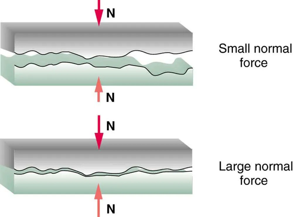
Figure 4.33 Two rough surfaces in contact have a much smaller area of actual contact than their total area. When there is a greater normal force as a result of a greater applied force, the area of actual contact increases as does friction. Image from OpenStax College Physics 2e, CC-BY 4.0
Image Description
The image consists of two side-by-side diagrams depicting surfaces under normal forces:
1. Top Diagram:
– Two surfaces are in contact, represented with a zigzag line to illustrate roughness.
– A downward red arrow labeled “N” indicates a small normal force is applied.
– An upward red arrow labeled “N” reflects equal reaction force.
– The caption on the right reads “Small normal force.”
2. Bottom Diagram:
– Similar depiction of two surfaces in contact with a zigzag line to show roughness.
– A larger downward red arrow labeled “N” signifies a large normal force.
– Correspondingly, a large upward red arrow labeled “N” represents the reaction force.
– The caption on the right reads “Large normal force.”
These diagrams illustrate the concept of normal force and its effect on contact surfaces.
But the atomic-scale view promises to explain far more than the simpler features of friction. The mechanism for how heat is generated is now being determined. In other words, why do surfaces get warmer when rubbed? Essentially, atoms are linked with one another to form lattices. When surfaces rub, the surface atoms adhere and cause atomic lattices to vibrate—essentially creating sound waves that penetrate the material. The sound waves diminish with distance and their energy is converted into heat. Chemical reactions that are related to frictional wear can also occur between atoms and molecules on the surfaces. Figure 4.34 shows how the tip of a probe drawn across another material is deformed by atomic-scale friction. The force needed to drag the tip can be measured and is found to be related to shear stress, which will be discussed later in this chapter. The variation in shear stress is remarkable (more than a factor of [latex]\text{10}^{\text{12}}[/latex]
) and difficult to predict theoretically, but shear stress is yielding a fundamental understanding of a large-scale phenomenon known since ancient times—friction.
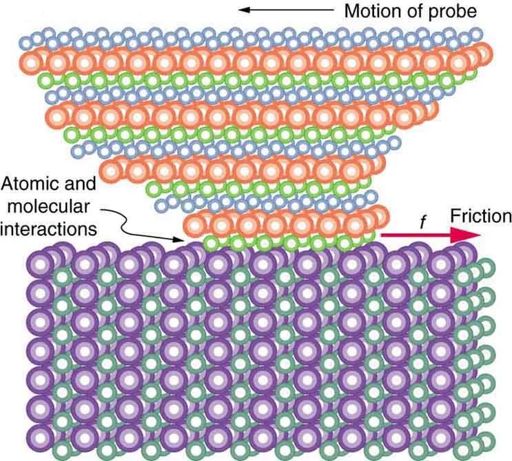
Figure 4.34 The tip of a probe is deformed sideways by frictional force as the probe is dragged across a surface. Measurements of how the force varies for different materials are yielding fundamental insights into the atomic nature of friction. Image from OpenStax College Physics 2e, CC-BY 4.0
Image Description
The image is a diagram illustrating atomic and molecular interactions between two surfaces, commonly used in explanations of friction at a microscopic level.
– Layers and Colors:
– The top part of the diagram consists of multiple rows of circles in different colors, including blue, orange, and green, representing atoms or molecules.
– The bottom layer consists of rows of circles colored in purple and green.
– Motion and Friction Arrows:
– An arrow labeled “Motion of probe” points to the left, indicating the direction of movement for the upper layers.
– Another arrow labeled “Friction” with the letter “f” points to the right, showing the direction of the frictional force acting against the movement of the probe.
– Labels:
– There is a label pointing to the interaction zone between the upper and lower layers, stating “Atomic and molecular interactions.”
This diagram is a schematic portrayal of how friction arises from the interaction between atomic or molecular layers when one surface moves over another.
PhET Explorations
Forces and Motion
Explore the forces at work when you try to push a filing cabinet. Create an applied force and see the resulting friction force and total force acting on the cabinet. Charts show the forces, position, velocity, and acceleration vs. time. Draw a free-body diagram of all the forces (including gravitational and normal forces).
