4.5 Normal, Tension, and Other Examples of Forces
Learning Objectives
By the end of this section, you will be able to:
- Define normal and tension forces.
- Apply Newton’s laws of motion to solve problems involving a variety of forces.
- Use trigonometric identities to resolve weight into components.
Forces are given many names, such as push, pull, thrust, lift, weight, friction, and tension. Traditionally, forces have been grouped into several categories and given names relating to their source, how they are transmitted, or their effects. The most important of these categories are discussed in this section, together with some interesting applications. Further examples of forces are discussed later in this text.
Normal Force
Weight (also called force of gravity) is a pervasive force that acts at all times and must be counteracted to keep an object from falling. You definitely notice that you must support the weight of a heavy object by pushing up on it when you hold it stationary, as illustrated in Figure 4.11(a). But how do inanimate objects like a table support the weight of a mass placed on them, such as shown in Figure 4.11(b)? When the bag of dog food is placed on the table, the table actually sags slightly under the load. This would be noticeable if the load were placed on a card table, but even rigid objects deform when a force is applied to them. Unless the object is deformed beyond its limit, it will exert a restoring force much like a deformed spring (or trampoline or diving board). The greater the deformation, the greater the restoring force. So when the load is placed on the table, the table sags until the restoring force becomes as large as the weight of the load. At this point the net external force on the load is zero. That is the situation when the load is stationary on the table. The table sags quickly, and the sag is slight so we do not notice it. But it is similar to the sagging of a trampoline when you climb onto it.
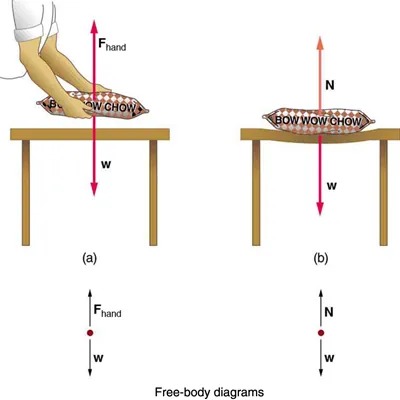
Figure 4.11 (a) The person holding the bag of dog food must supply an upward force [latex]\textbf{F}_{\text{hand}}[/latex] equal in magnitude and opposite in direction to the weight of the food [latex]\textbf{w}[/latex]. (b) The card table sags when the dog food is placed on it, much like a stiff trampoline. Elastic restoring forces in the table grow as it sags until they supply a force [latex]\textbf{N}[/latex] equal in magnitude and opposite in direction to the weight of the load. Image from OpenStax College Physics 2e, CC-BY 4.0
Image Description
The image features two diagrams demonstrating the concept of forces applied to a bag. Both diagrams show a bag labeled “BOW WOW CHOW” placed on a table.
– Diagram (a):
– A pair of hands is pressing down on the bag, causing it to compress.
– An arrow labeled “Fhand” points upwards, representing the force applied by the hands.
– An arrow labeled “w” points downwards, indicating the weight of the bag.
– Below the table, a free-body diagram shows a dot with an upward arrow labeled “Fhand” and a downward arrow labeled “w.”
– Diagram (b):
– The bag is shown without any external force being applied, allowing it to remain uncompressed but slightly deformed by its own weight.
– An arrow labeled “N” points upwards, which represents the normal force exerted by the table on the bag.
– An arrow labeled “w” points downwards, indicating the weight of the bag.
– Below the table, a free-body diagram shows a dot with an upward arrow labeled “N” and a downward arrow labeled “w.”
Below both diagrams, the text reads “Free-body diagrams.”
We must conclude that whatever supports a load, be it animate or not, must supply an upward force equal to the weight of the load, as we assumed in a few of the previous examples. If the force supporting a load is perpendicular to the surface of contact between the load and its support, this force is defined to be a normal force and here is given the symbol [latex]\textbf{N}[/latex]. (This is not the unit for force N.) The word normal means perpendicular to a surface. The normal force can be less than the object’s weight if the object is on an incline, as you will see in the next example.
Common Misconception: Normal Force (N) vs. Newton (N)
In this section we have introduced the quantity normal force, which is represented by the variable [latex]\textbf{N}[/latex]. This should not be confused with the symbol for the newton, which is also represented by the letter N. These symbols are particularly important to distinguish because the units of a normal force ([latex]\textbf{N}[/latex]) happen to be newtons (N). For example, the normal force [latex]\textbf{N}[/latex] that the floor exerts on a chair might be [latex]\textbf{N} = \text{100 N}[/latex]. One important difference is that normal force is a vector, while the newton is simply a unit. Be careful not to confuse these letters in your calculations! You will encounter more similarities among variables and units as you proceed in physics. Another example of this is the quantity work ([latex]W[/latex]) and the unit watts (W).
Example 4.5
Weight on an Incline, a Two-Dimensional Problem
Consider the skier on a slope shown in Figure 4.12. Her mass including equipment is 60.0 kg. (a) What is her acceleration if friction is negligible? (b) What is her acceleration if friction is known to be 45.0 N?
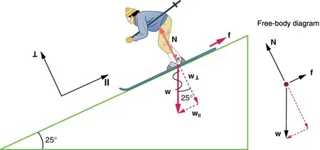
Figure 4.12 Since motion and friction are parallel to the slope, it is most convenient to project all forces onto a coordinate system where one axis is parallel to the slope and the other is perpendicular (axes shown to left of skier). [latex]\textbf{N}[/latex] is perpendicular to the slope and f is parallel to the slope, but [latex]\textbf{w}[/latex] has components along both axes, namely [latex]\textbf{w}_{\bot}[/latex] and [latex]\textbf{w}_{\parallel}[/latex]. [latex]\textbf{N}[/latex] is equal in magnitude to [latex]\textbf{w}_{\bot}[/latex], so that there is no motion perpendicular to the slope, but [latex]f[/latex] is less than [latex]w_{\parallel}[/latex], so that there is a downslope acceleration Image from OpenStax College Physics 2e, CC-BY 4.0
Image Description
The image shows a skier descending a slope inclined at 25 degrees. The skier is leaning forward and using ski poles for balance. The diagram is labeled as a “Free-body diagram.”
To the left, there is a depiction of the slope with three arrows indicating forces. The arrow labeled “N” represents the normal force perpendicular to the slope. The force of friction, labeled “f,” acts parallel to the slope and pointed uphill. The weight of the skier, labeled “W,” is shown with a vector pointing straight down. The weight vector is decomposed into two components: “W⊥” is perpendicular to the slope and “W‖” is parallel to the slope.
On the right, a simplified free-body diagram shows these forces without the skier: “N” points perpendicularly from the slope, “W” points downward, and “f” points up the slope. The weight vector “W” is shown decomposed into its components with “W⊥” and “W‖” forming a 25-degree angle with each other.
These diagrams visually represent the forces acting on the skier as they move down the slope.
Strategy
This is a two-dimensional problem, since the forces on the skier (the system of interest) are not parallel. The approach we have used in two-dimensional kinematics also works very well here. Choose a convenient coordinate system and project the vectors onto its axes, creating two connected one-dimensional problems to solve. The most convenient coordinate system for motion on an incline is one that has one coordinate parallel to the slope and one perpendicular to the slope. (Remember that motions along mutually perpendicular axes are independent.) We use the symbols [latex]\bot[/latex] and [latex]\parallel[/latex] to represent perpendicular and parallel, respectively. This choice of axes simplifies this type of problem, because there is no motion perpendicular to the slope and because friction is always parallel to the surface between two objects. The only external forces acting on the system are the skier’s weight, friction, and the support of the slope, respectively labeled [latex]\textbf{w}[/latex], [latex]\textbf{f}[/latex], and [latex]\textbf{N}[/latex] in Figure 4.12. [latex]\textbf{N}[/latex] is always perpendicular to the slope, and [latex]\textbf{f}[/latex] is parallel to it. But [latex]\textbf{w}[/latex] is not in the direction of either axis, and so the first step we take is to project it into components along the chosen axes, defining [latex]w_{\parallel}[/latex] to be the component of weight parallel to the slope and [latex]w_{\bot}[/latex] the component of weight perpendicular to the slope. Once this is done, we can consider the two separate problems of forces parallel to the slope and forces perpendicular to the slope.
Solution
The magnitude of the component of the weight parallel to the slope is [latex]w_{\parallel} = \mathit{w} \text{sin} \left(\right. \text{25}º \left.\right) = \mathit{mg} \text{sin} \left(\right. \text{25}º \left.\right)[/latex], and the magnitude of the component of the weight perpendicular to the slope is [latex]w_{\bot} = \mathit{w} \text{cos} \left(\right. \text{25}º \left.\right) = \mathit{mg} \text{cos} \left(\right. \text{25}º \left.\right)[/latex].
(a) Neglecting friction. Since the acceleration is parallel to the slope, we need only consider forces parallel to the slope. (Forces perpendicular to the slope add to zero, since there is no acceleration in that direction.) The forces parallel to the slope are the amount of the skier’s weight parallel to the slope [latex]w_{\parallel}[/latex] and friction [latex]f[/latex]. Using Newton’s second law, with subscripts to denote quantities parallel to the slope, [latex]a_{\parallel} = \frac{F_{\text{net } \parallel}}{m}[/latex]
where [latex]F_{\text{net } \parallel} = w_{\parallel} = \text{mg} \text{sin} \left(\right. \text{25}º \left.\right)[/latex], assuming no friction for this part, so that
[latex]a_{\parallel} = \frac{F_{\text{net } \parallel}}{m} = \frac{\text{mg} \text{sin} \left(\right. \text{25}º \left.\right)}{m} = g \text{sin} \left(\right. \text{25}º \left.\right)[/latex]
[latex]\left(\right. 9.80 \text{ m}/\text{s}^{2} \left.\right) \left(\right. 0.4226 \left.\right) = 4.14 \text{m}/\text{s}^{2}[/latex]
is the acceleration.
(b) Including friction. We now have a given value for friction, and we know its direction is parallel to the slope and it opposes motion between surfaces in contact. So the net external force is now
[latex]F_{\text{net } \parallel} = w_{\parallel} - f ,[/latex]
and substituting this into Newton’s second law, [latex]a_{\parallel} = \frac{F_{\text{net } \parallel}}{m}[/latex], gives
[latex]a_{\parallel} = \frac{F_{\text{net } \mid \mid}}{m} = \frac{w_{\parallel} - f}{m} = \frac{\text{mg} \text{sin} \left(\right. \text{25}º \left.\right) - f}{m} .[/latex]
We substitute known values to obtain
[latex]a_{\parallel} = \frac{\left(\right. \text{60} . \text{0 kg} \left.\right) \left(\right. 9 . \text{80 m}/\text{s}^{2} \left.\right) \left(\right. 0 . \text{4226} \left.\right) - \text{45} . \text{0 N}}{\text{60} . \text{0 kg}} ,[/latex]
which yields
[latex]a_{\parallel} = 3 . \text{39 m}/\text{s}^{2} ,[/latex]
which is the acceleration parallel to the incline when there is 45.0 N of opposing friction.
Discussion
Since friction always opposes motion between surfaces, the acceleration is smaller when there is friction than when there is none. In fact, it is a general result that if friction on an incline is negligible, then the acceleration down the incline is [latex]a = g \text{sin} \theta[/latex], regardless of mass. This is related to the previously discussed fact that all objects fall with the same acceleration in the absence of air resistance. Similarly, all objects, regardless of mass, slide down a frictionless incline with the same acceleration (if the angle is the same).
Resolving Weight into Components
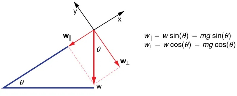
Figure 4.13 An object rests on an incline that makes an angle θ with the horizontal. Image from OpenStax College Physics 2e, CC-BY 4.0
Image Description
The image is a diagram illustrating the decomposition of a weight vector w on an inclined plane. The inclined plane is represented as a blue triangle with the angle θ at the bottom left corner. The weight vector w is shown as a red arrow pointing downwards, perpendicular to the horizontal ground.
There are two components of the weight vector depicted:
- w∥: Parallel to the inclined plane, shown as a red arrow pointing down the plane.
- w⊥: Perpendicular to the inclined plane, shown as a red arrow pointing directly into the inclined surface.
The axis is labeled with x pointing up the incline and y perpendicular to it.
To the right of the diagram, there are equations representing the components of the weight vector:
- w∥ = w sin(θ) = mg sin(θ)
- w⊥ = w cos(θ) = mg cos(θ)
Here, w is the weight of the object, m is the mass, and g is the acceleration due to gravity.
When an object rests on an incline that makes an angle [latex]\theta[/latex] with the horizontal, the force of gravity acting on the object is divided into two components: a force acting perpendicular to the plane, [latex]\textbf{w}_{\bot}[/latex], and a force acting parallel to the plane, [latex]\textbf{w}_{\parallel}[/latex]. The perpendicular force of weight, [latex]\textbf{w}_{\bot}[/latex], is typically equal in magnitude and opposite in direction to the normal force, [latex]\textbf{N}[/latex]. The force acting parallel to the plane, [latex]\textbf{w}_{\parallel}[/latex], causes the object to accelerate down the incline. The force of friction, [latex]\mathbf{f}[/latex], opposes the motion of the object, so it acts upward along the plane.
It is important to be careful when resolving the weight of the object into components. If the angle of the incline is at an angle [latex]\theta[/latex] to the horizontal, then the magnitudes of the weight components are
[latex]w_{\parallel} = w \text{sin} \left(\right. \theta \left.\right) = \text{mg} \text{sin} \left(\right. \theta \left.\right)[/latex]
and
[latex]w_{\bot} = w \text{cos} \left(\right. \theta \left.\right) = \text{mg} \text{cos} \left(\right. \theta \left.\right) .[/latex]
Instead of memorizing these equations, it is helpful to be able to determine them from reason. To do this, draw the right triangle formed by the three weight vectors. Notice that the angle [latex]\theta[/latex] of the incline is the same as the angle formed between [latex]\textbf{w}[/latex] and [latex]\textbf{w}_{\bot}[/latex]. Knowing this property, you can use trigonometry to determine the magnitude of the weight components:
[latex]\begin{eqnarray*}\text{cos} \left(\right. \theta \left.\right) & = & \frac{w_{\bot}}{w} \\ w_{\bot} & = & w \text{cos} \left(\right. \theta \left.\right) = \text{mg} \text{cos} \left(\right. \theta \left.\right)\end{eqnarray*}[/latex]
[latex]\begin{eqnarray*}\text{sin} \left(\right. \theta \left.\right) & = & \frac{w_{\parallel}}{w} \\ w_{\parallel} & = & w \text{sin} \left(\right. \theta \left.\right) = \text{mg} \text{sin} \left(\right. \theta \left.\right)\end{eqnarray*}[/latex]
Take-Home Experiment: Force Parallel
To investigate how a force parallel to an inclined plane changes, find a rubber band, some objects to hang from the end of the rubber band, and a board you can position at different angles. How much does the rubber band stretch when you hang the object from the end of the board? Now place the board at an angle so that the object slides off when placed on the board. How much does the rubber band extend if it is lined up parallel to the board and used to hold the object stationary on the board? Try two more angles. What does this show?
Tension
A tension is a force along the length of a medium, especially a force carried by a flexible medium, such as a rope or cable. The word “tension” comes from a Latin word meaning “to stretch.” Not coincidentally, the flexible cords that carry muscle forces to other parts of the body are called tendons. Any flexible connector, such as a string, rope, chain, wire, or cable, can exert pulls only parallel to its length; thus, a force carried by a flexible connector is a tension with direction parallel to the connector. It is important to understand that tension is a pull in a connector. In contrast, consider the phrase: “You can’t push a rope.” The tension force pulls outward along the two ends of a rope.
Consider a person holding a mass on a rope as shown in Figure 4.14.
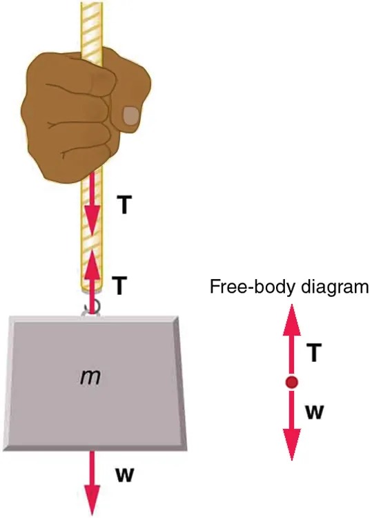
Figure 4.14 When a perfectly flexible connector (one requiring no force to bend it) such as this rope transmits a force [latex]\textbf{T}[/latex], that force must be parallel to the length of the rope, as shown. The pull such a flexible connector exerts is a tension. Note that the rope pulls with equal force but in opposite directions on the hand and the supported mass (neglecting the weight of the rope). This is an example of Newton’s third law. The rope is the medium that carries the equal and opposite forces between the two objects. The tension anywhere in the rope between the hand and the mass is equal. Once you have determined the tension in one location, you have determined the tension at all locations along the rope. Image from OpenStax College Physics 2e, CC-BY 4.0
Image Description
The image shows a hand gripping a rope that is connected to a rectangular block labeled with “m”. There are arrows and labels indicating forces acting on the system. The following elements are present:
– A hand is grasping a rope, which is vertical.
– The rope is attached to the top of a rectangular block with the mass labeled as “m”.
– Two upward arrows, labeled “T”, are drawn along the rope, signifying the tension force exerted by the rope at different points.
– A downward arrow labeled “w” is shown at the bottom of the block, representing the weight of the block.
– On the right side of the image, there is a free-body diagram:
– A small dot represents the object (the block).
– An upward arrow labeled “T” shows the tension force.
– A downward arrow labeled “w” shows the weight force.
– The term “Free-body diagram” is written next to the simplified representation to explain the forces acting on the block.
Tension in the rope must equal the weight of the supported mass, as we can prove using Newton’s second law. If the 5.00-kg mass in the figure is stationary, then its acceleration is zero, and thus [latex]\textbf{F}_{\text{net}} = 0[/latex]. The only external forces acting on the mass are its weight [latex]\textbf{w}[/latex] and the tension [latex]\textbf{T}[/latex] supplied by the rope. Thus,
[latex]F_{\text{net}} = T - w = 0 ,[/latex]
where [latex]T[/latex] and [latex]w[/latex] are the magnitudes of the tension and weight and their signs indicate direction, with up being positive here. Thus, just as you would expect, the tension equals the weight of the supported mass:
[latex]T = w = \text{mg} .[/latex]
For a 5.00-kg mass, then (neglecting the mass of the rope) we see that
[latex]T = \text{mg} = \left(\right. \text{5}.\text{00 kg} \left.\right) \left(\right. 9 . \text{80 m}/\text{s}^{2} \left.\right) = \text{49}.\text{0 N} .[/latex]
If we cut the rope and insert a spring, the spring would extend a length corresponding to a force of 49.0 N, providing a direct observation and measure of the tension force in the rope.
Flexible connectors are often used to transmit forces around corners, such as in a hospital traction system, a finger joint, or a bicycle brake cable. If there is no friction, the tension is transmitted undiminished. Only its direction changes, and it is always parallel to the flexible connector. This is illustrated in Figure 4.15 (a) and (b).
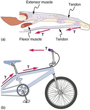
Figure 4.15 (a) Tendons in the finger carry force [latex]\textbf{T}[/latex] from the muscles to other parts of the finger, usually changing the force’s direction, but not its magnitude (the tendons are relatively friction free). (b) The brake cable on a bicycle carries the tension [latex]\textbf{T}[/latex] from the handlebars to the brake mechanism. Again, the direction but not the magnitude of [latex]\textbf{T}[/latex] is changed. Image from OpenStax College Physics 2e, CC-BY 4.0
Image Description
The image consists of two diagrams labeled (a) and (b), illustrating concepts related to tension.
—
**Diagram (a): Anatomy of Muscles and Tendons**
– The diagram shows a side view of a human arm focusing on the muscles and tendons.
– Extensor Muscle: Located at the top, indicated by a label.
– Flexor Muscle: Found below the extensor muscle, also labeled.
– Tendons: Connect muscles to the bones, with arrows indicating the direction of tension.
– Tension (T): Represented by red arrows showing the forces at work in the muscles and tendons.
—
Diagram (b): Bicycle Structure
– The diagram displays a side view of a bicycle.
– Main components shown:
– Handlebars: Labeled, with an arrow pointing to the right.
– Frame: Includes the top tube, seat tube, and down tube.
– Pedals and Chainwheel: Situated towards the bottom of the frame.
– Tension (T): Highlighted by red arrows indicating the direction of tension along the frame’s components.
—
Both diagrams use red arrows to represent the concept of tension within their respective contexts, emphasizing how forces are at play in both biological and mechanical systems.
Example 4.6
What Is the Tension in a Tightrope?
Calculate the tension in the wire supporting the 70.0-kg tightrope walker shown in Figure 4.16.
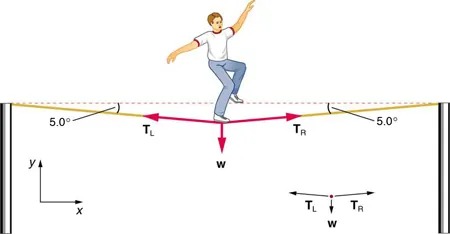
Figure 4.16 The weight of a tightrope walker causes a wire to sag by 5.0 degrees. The system of interest here is the point in the wire at which the tightrope walker is standing. Image from OpenStax College Physics 2e, CC-BY 4.0
Image Description
The image illustrates the physics of a person balancing on a tightrope. Here’s a breakdown of the elements in the image:
– Person on Tightrope: A person is standing in the center of a tightrope, arms outstretched for balance.
– Tightrope: The tightrope is depicted as a straight line with slight angles at both ends where it connects to supports. The angles are labeled as 5.0 degrees.
– Forces:
– There are three forces shown acting on the rope at the point where the person stands: two tensile forces and the weight of the person.
– Left Tension (TL): An arrow is labeled TL pointing diagonally upwards to the left.
– Right Tension (TR): An arrow is labeled TR pointing diagonally upwards to the right.
– Weight (w): An arrow labeled w points directly downwards towards the tightrope.
– Angle and Direction:
– Both sides of the rope are angled upward from the horizontal by 5.0 degrees, with arrows indicating the direction of tension forces.
– Graphical Elements:
– A small coordinate system is shown at the bottom left corner with x and y axes labeled.
– Beside the person balancing, there is a small diagram repeating the three force arrows (TL, TR, and w) to indicate their directions and interactions.
This visual representation helps in understanding the equilibrium and balance involved in tightrope walking, focusing on the tension and gravitational forces at play.
Strategy
As you can see in the figure, the wire is not perfectly horizontal (it cannot be!), but is bent under the person’s weight. Thus, the tension on either side of the person has an upward component that can support his weight. As usual, forces are vectors represented pictorially by arrows having the same directions as the forces and lengths proportional to their magnitudes. The system is the tightrope walker, and the only external forces acting on him are his weight [latex]\textbf{w}[/latex] and the two tensions [latex]\textbf{T}_{\text{L}}[/latex] (left tension) and [latex]\textbf{T}_{\text{R}}[/latex] (right tension), as illustrated. It is reasonable to neglect the weight of the wire itself. The net external force is zero since the system is stationary. A little trigonometry can now be used to find the tensions. One conclusion is possible at the outset—we can see from part (b) of the figure that the magnitudes of the tensions [latex]T_{\text{L}}[/latex] and [latex]T_{\text{R}}[/latex] must be equal. This is because there is no horizontal acceleration in the rope, and the only forces acting to the left and right are [latex]T_{\text{L}}[/latex] and [latex]T_{R}[/latex]. Thus, the magnitude of those forces must be equal so that they cancel each other out.
Whenever we have two-dimensional vector problems in which no two vectors are parallel, the easiest method of solution is to pick a convenient coordinate system and project the vectors onto its axes. In this case the best coordinate system has one axis horizontal and the other vertical. We call the horizontal the [latex]x[/latex]-axis and the vertical the [latex]y[/latex]-axis.
Solution
First, we need to resolve the tension vectors into their horizontal and vertical components. It helps to draw a new free-body diagram showing all of the horizontal and vertical components of each force acting on the system.
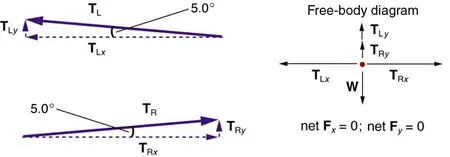
Figure 4.17 When the vectors are projected onto vertical and horizontal axes, their components along those axes must add to zero, since the tightrope walker is stationary. The small angle results in [latex]T[/latex] being much greater than [latex]w[/latex]. Image from OpenStax College Physics 2e, CC-BY 4.0
Image Description
The image consists of two sets of diagrams related to physics, specifically forces and tension angles.
The left side of the image shows two diagrams with inclined arrows representing forces on a plane tilted at a 5-degree angle. Each diagram includes:
- The top diagram displays the force TL (left tension) with its vertical component TLy pointing upwards and its horizontal component TLx pointing to the right along the plane.
- The bottom diagram shows the force TR (right tension) with its vertical component TRy pointing upwards and its horizontal component TRx pointing to the left along the plane.
The right side of the image features a labeled free-body diagram that summarizes the forces in a single coordinate system:
- An upward pointing arrow labeled TLy.
- A downward pointing arrow labeled W (weight).
- A rightward pointing arrow labeled TLx.
- A leftward pointing arrow labeled TRx.
- An upward pointing arrow labeled TRy.
Below the free-body diagram, there are notes indicating the conditions:
net Fx = 0; net Fy = 0, signifying that the net forces in both the x and y directions are zero, implying equilibrium.
Consider the horizontal components of the forces (denoted with a subscript [latex]x[/latex]):
[latex]F_{\text{net } x} = T_{\text{L} x} - T_{\text{R} x} .[/latex]
The net external horizontal force [latex]F_{\text{net } x} = 0[/latex], since the person is stationary. Thus,
[latex]\begin{eqnarray*}F_{\text{net } x} = 0 & = & T_{\text{L} x} - T_{\text{R} x} \\ T_{\text{L} x} & = & T_{\text{R} x} .\end{eqnarray*}[/latex]
Now, observe Figure 4.17. You can use trigonometry to determine the magnitude of [latex]T_{\text{L}}[/latex] and [latex]T_{\text{R}}[/latex]. Notice that:
[latex]\begin{eqnarray*}\text{cos} \left(\right. 5.0º \left.\right) & = & \frac{T_{\text{L} x}}{T_{\text{L}}} \\ T_{\text{L} x} & = & T_{\text{L}} \text{cos} \left(\right. 5.0º \left.\right) \\ \text{cos} \left(\right. 5.0º \left.\right) & = & \frac{T_{\text{R} x}}{T_{\text{R}}} \\ T_{\text{R} x} & = & T_{\text{R}} \text{cos} \left(\right. 5.0º \left.\right) .\end{eqnarray*}[/latex]
Equating [latex]T_{\text{L} x}[/latex] and [latex]T_{\text{R} x}[/latex]:
[latex]T_{\text{L}} \text{cos} \left(\right. 5.0º \left.\right) = T_{\text{R}} \text{cos} \left(\right. 5.0º \left.\right) .[/latex]
Thus,
[latex]T_{\text{L}} = T_{\text{R}} = T ,[/latex]
as predicted. Now, considering the vertical components (denoted by a subscript [latex]y[/latex]), we can solve for [latex]T[/latex]. Again, since the person is stationary, Newton’s second law implies that net [latex]F_{y} = 0[/latex]. Thus, as illustrated in the free-body diagram in Figure 4.17,
[latex]F_{\text{net } y} = T_{\text{L} y} + T_{\text{R} y} - w = 0 .[/latex]
Observing Figure 4.17, we can use trigonometry to determine the relationship between [latex]T_{\text{L} y}[/latex], [latex]T_{\text{R} y}[/latex], and [latex]T[/latex]. As we determined from the analysis in the horizontal direction, [latex]T_{\text{L}} = T_{\text{R}} = T[/latex]:
[latex]\begin{eqnarray*}\text{sin} \left(\right. 5.0º \left.\right) & = & \frac{T_{\text{L} y}}{T_{\text{L}}} \\ T_{\text{L} y} = T_{\text{L}} \text{sin} \left(\right. 5.0º \left.\right) & = & T \text{sin} \left(\right. 5.0º \left.\right) \\ \text{sin} \left(\right. 5.0º \left.\right) & = & \frac{T_{\text{R} y}}{T_{\text{R}}} \\ T_{\text{R} y} = T_{\text{R}} \text{sin} \left(\right. 5.0º \left.\right) & = & T \text{sin} \left(\right. 5.0º \left.\right) .\end{eqnarray*}[/latex]
Now, we can substitute the values for [latex]T_{\text{L} y}[/latex] and [latex]T_{\text{R} y}[/latex], into the net force equation in the vertical direction:
[latex]\begin{eqnarray*}F_{\text{net } y} = T_{\text{L} y} + T_{\text{R} y} - w &=& 0 \\ T \text{sin} \left(\right. 5.0º \left.\right) + T \text{sin} \left(\right. 5.0º \left.\right) - w &=& 0 \\ 2 T \text{sin} \left(\right. 5.0º \left.\right) - w & = & 0 \\ 2 T \text{sin} \left(\right. 5.0º \left.\right) & = & w\end{eqnarray*}[/latex]
and
[latex]T = \frac{w}{2 \text{sin} \left(\right. 5.0º \left.\right)} = \frac{\text{mg}}{2 \text{sin} \left(\right. 5.0º \left.\right)} ,[/latex]
so that
[latex]T = \frac{\left(\right. \text{70} . \text{0 kg} \left.\right) \left(\right. 9 . \text{80 m}/\text{s}^{2} \left.\right)}{2 \left(\right. 0 . \text{0872} \left.\right)} ,[/latex]
and the tension is
[latex]T = \text{3900 N} .[/latex]
Discussion
Note that the vertical tension in the wire acts as a normal force that supports the weight of the tightrope walker. The tension is almost six times the 686-N weight of the tightrope walker. Since the wire is nearly horizontal, the vertical component of its tension is only a small fraction of the tension in the wire. The large horizontal components are in opposite directions and cancel, and so most of the tension in the wire is not used to support the weight of the tightrope walker.
If we wish to create a very large tension, all we have to do is exert a force perpendicular to a flexible connector, as illustrated in Figure 4.18. As we saw in the last example, the weight of the tightrope walker acted as a force perpendicular to the rope. We saw that the tension in the roped related to the weight of the tightrope walker in the following way:
[latex]T = \frac{w}{2 \text{sin} \left(\right. \theta \left.\right)} .[/latex]
We can extend this expression to describe the tension [latex]T[/latex] created when a perpendicular force ([latex]\textbf{F}_{\bot}[/latex]) is exerted at the middle of a flexible connector:
[latex]T = \frac{F_{\bot}}{2 \text{sin} \left(\right. \theta \left.\right)} .[/latex]
Note that [latex]\theta[/latex] is the angle between the horizontal and the bent connector. In this case, [latex]T[/latex] becomes very large as [latex]\theta[/latex] approaches zero. Even the relatively small weight of any flexible connector will cause it to sag, since an infinite tension would result if it were horizontal (i.e.,
[latex]\theta = 0[/latex] and [latex]\text{sin} \theta = 0[/latex]). (See Figure 4.18.)
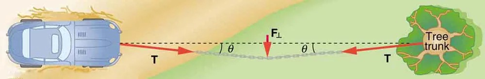
Figure 4.18 We can create a very large tension in the chain by pushing on it perpendicular to its length, as shown. Suppose we wish to pull a car out of the mud when no tow truck is available. Each time the car moves forward, the chain is tightened to keep it as nearly straight as possible. The tension in the chain is given by [latex]T = \frac{F_{\bot}}{2 \text{sin} \left(\right. \theta \left.\right)}[/latex] ; since [latex]\theta[/latex] is small, [latex]T[/latex] is very large. This situation is analogous to the tightrope walker shown in , except that the tensions shown here are those transmitted to the car and the tree rather than those acting at the point where [latex]\textbf{F}_{\bot}[/latex] is applied. Image from OpenStax College Physics 2e, CC-BY 4.0
Image Description
The image depicts a diagram of a blue car stuck in sand, connected by a chain to a tree trunk. The car is on the left side, and the tree is on the right. The chain is under tension and forms two equal angles, labeled as θ (theta), with the ground. There are red arrows labeled “T” representing tension forces pointing along the chain from both the car and the tree trunk. At the midpoint of the chain, there is a downward arrow labeled “F₁” representing a force. The ground surrounding the tree trunk is green, while the area around the car is sandy.
Extended Topic: Real Forces and Inertial Frames
There is another distinction among forces in addition to the types already mentioned. Some forces are real, whereas others are not. Real forces are those that have some physical origin, such as the gravitational pull. Contrastingly, fictitious forces are those that arise simply because an observer is in an accelerating frame of reference, such as one that rotates (like a merry-go-round) or undergoes linear acceleration (like a car slowing down). For example, if a satellite is heading due north above Earth’s northern hemisphere, then to an observer on Earth it will appear to experience a force to the west that has no physical origin. Of course, what is happening here is that Earth is rotating toward the east and moves east under the satellite. In Earth’s frame this looks like a westward force on the satellite, or it can be interpreted as a violation of Newton’s first law (the law of inertia). An inertial frame of reference is one in which all forces are real and, equivalently, one in which Newton’s laws have the simple forms given in this chapter.
Earth’s rotation is slow enough that Earth is nearly an inertial frame. You ordinarily must perform precise experiments to observe fictitious forces and the slight departures from Newton’s laws, such as the effect just described. On the large scale, such as for the rotation of weather systems and ocean currents, the effects can be easily observed.
The crucial factor in determining whether a frame of reference is inertial is whether it accelerates or rotates relative to a known inertial frame. Unless stated otherwise, all phenomena discussed in this text are considered in inertial frames.
All the forces discussed in this section are real forces, but there are a number of other real forces, such as lift and thrust, that are not discussed in this section. They are more specialized, and it is not necessary to discuss every type of force. It is natural, however, to ask where the basic simplicity we seek to find in physics is in the long list of forces. Are some more basic than others? Are some different manifestations of the same underlying force? The answer to both questions is yes, as will be seen in the next (extended) section and in the treatment of modern physics later in the text.
PhET Explorations
Forces in 1 Dimension
Explore the forces at work when you try to push a filing cabinet. Create an applied force and see the resulting friction force and total force acting on the cabinet. Charts show the forces, position, velocity, and acceleration vs. time. View a free-body diagram of all the forces (including gravitational and normal forces).
