2.5 Motion Equations for Constant Acceleration in One Dimension
Learning Objectives
By the end of this section, you will be able to:
- Calculate displacement of an object that is not accelerating, given initial position and velocity.
- Calculate final velocity of an accelerating object, given initial velocity, acceleration, and time.
- Calculate displacement and final position of an accelerating object, given initial position, initial velocity, time, and acceleration.
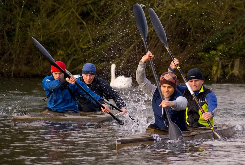
Figure 2.24 Kinematic equations can help us describe and predict the motion of moving objects such as these kayaks racing in Newbury, England. Image from OpenStax College Physics 2e, CC-BY 4.0
We might know that the greater the acceleration of, say, a car moving away from a stop sign, the greater the displacement in a given time. But we have not developed a specific equation that relates acceleration and displacement. In this section, we develop some convenient equations for kinematic relationships, starting from the definitions of displacement, velocity, and acceleration already covered.
Notation: t, x, v, a
First, let us make some simplifications in notation. Taking the initial time to be zero, as if time is measured with a stopwatch, is a great simplification. Since elapsed time is [latex]Δ t = t_{f} - t_{0}[/latex], taking [latex]t_{0} = 0[/latex] means that [latex]Δ t = t_{f}[/latex], the final time on the stopwatch. When initial time is taken to be zero, we use the subscript 0 to denote initial values of position and velocity. That is, [latex]x_{0}[/latex] is the initial position and [latex]v_{0}[/latex] is the initial velocity. We put no subscripts on the final values. That is, [latex]t[/latex] is the final time, [latex]x[/latex] is the final position, and [latex]v[/latex] is the final velocity. This gives a simpler expression for elapsed time—now, [latex]Δ t = t[/latex]. It also simplifies the expression for displacement, which is now [latex]Δ x = x - x_{0}[/latex]. Also, it simplifies the expression for change in velocity, which is now [latex]Δ v = v - v_{0}[/latex]. To summarize, using the simplified notation, with the initial time taken to be zero,
[latex]\begin{matrix} Δ t & = & t \\ Δ x & = & x - x_{0} \\ Δ v & = & v - v_{0} \end{matrix}[/latex]
where the subscript 0 denotes an initial value and the absence of a subscript denotes a final value in whatever motion is under consideration.
We now make the important assumption that acceleration is constant. This assumption allows us to avoid using calculus to find instantaneous acceleration. Since acceleration is constant, the average and instantaneous accelerations are equal. That is,
[latex]\overset{-}{a} = a = \text{constant} ,[/latex]
so we use the symbol [latex]a[/latex] for acceleration at all times. Assuming acceleration to be constant does not seriously limit the situations we can study nor degrade the accuracy of our treatment. For one thing, acceleration is constant in a great number of situations. Furthermore, in many other situations we can accurately describe motion by assuming a constant acceleration equal to the average acceleration for that motion. Finally, in motions where acceleration changes drastically, such as a car accelerating to top speed and then braking to a stop, the motion can be considered in separate parts, each of which has its own constant acceleration.
Solving for Displacement ([latex]{\color{white}Δx}[/latex]) and Final Position ([latex]{\color{white}x}[/latex]) from Average Velocity when Acceleration ([latex]{\color{white}a}[/latex]) is Constant
To get our first two new equations, we start with the definition of average velocity:
[latex]\overset{-}{v} = \frac{Δ x}{Δ t} .[/latex]
Substituting the simplified notation for [latex]Δ x[/latex] and [latex]Δ t[/latex] yields
[latex]\overset{-}{v} = \frac{x - x_{0}}{t} .[/latex]
Solving for [latex]x[/latex] yields
[latex]x = x_{0} + \overset{-}{v} t ,[/latex]
where the average velocity is
[latex]\overset{-}{v} = \frac{v_{0} + v}{2} \left(\right. \text{constant } a \left.\right) .[/latex]
The equation [latex]\overset{-}{v} = \frac{v_{0} + v}{2}[/latex] reflects the fact that, when acceleration is constant, [latex]v[/latex] is just the simple average of the initial and final velocities. For example, if you steadily increase your velocity (that is, with constant acceleration) from 30 to 60 km/h, then your average velocity during this steady increase is 45 km/h. Using the equation [latex]\overset{-}{v} = \frac{v_{0} + v}{2}[/latex] to check this, we see that
[latex]\overset{-}{v} = \frac{v_{0} + v}{2} = \frac{\text{30 km}/\text{h} + \text{60 km}/\text{h}}{2} = \text{45 km}/\text{h},[/latex]
which seems logical.
Example 2.8
Calculating Displacement: How Far does the Jogger Run?
A jogger runs down a straight stretch of road with an average velocity of 4.00 m/s for 2.00 min. What is his final position, taking his initial position to be zero?
Strategy
Draw a sketch.
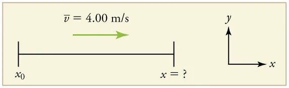
Figure 2.25 Image from OpenStax College Physics 2e, CC-BY 4.0
Image Description
The image is a diagram representing motion along a straight path, depicted in a horizontal plane with an x-y coordinate system for orientation.
On the left side of the diagram, there is a horizontal line segment, representing a path with two endpoints:
- The left endpoint is labeled x0, indicating the initial position.
- The right endpoint is labeled x = ?, symbolizing the final position which is unknown.
An arrow is drawn above the line segment pointing from left to right, symbolizing motion in the positive x-direction. Above the arrow, the velocity is specified as v̅ = 4.00 m/s, indicating constant speed.
To the right of the path, there is an x-y coordinate system. The x-axis is parallel to the path, extending horizontally to the right, and the y-axis is vertical, pointing upwards.
The final position [latex]x[/latex] is given by the equation
[latex]x = x_{0} + \overset{-}{v} t .[/latex]
To find [latex]x[/latex], we identify the values of [latex]x_{0}[/latex], [latex]\overset{-}{v}[/latex], and [latex]t[/latex] from the statement of the problem and substitute them into the equation.
Solution
1. Identify the knowns. [latex]\overset{-}{v} = 4 . \text{00 m}/\text{s}[/latex], [latex]Δ t = 2.00 \text{min}[/latex], and [latex]x_{0} = \text{0 m}[/latex].
2. Enter the known values into the equation.
[latex]x = x_{0} + \overset{-}{v} t = 0 + \left(4 . \text{00 m}/\text{s}\right) \left(\text{120 s}\right) = \text{480 m}[/latex]
Discussion
Velocity and final displacement are both positive, which means they are in the same direction.
The equation [latex]x = x_{0} + \overset{-}{v} t[/latex] gives insight into the relationship between displacement, average velocity, and time. It shows, for example, that displacement is a linear function of average velocity. (By linear function, we mean that displacement depends on [latex]\overset{-}{v}[/latex] rather than on [latex]\overset{-}{v}[/latex] raised to some other power, such as [latex]\left(\overset{-}{v}\right)^{2}[/latex]. When graphed, linear functions look like straight lines with a constant slope.) On a car trip, for example, we will get twice as far in a given time if we average 90 km/h than if we average 45 km/h.
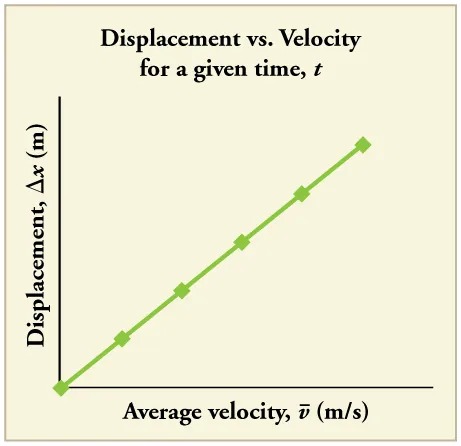
Figure 2.26 There is a linear relationship between displacement and average velocity. For a given time [latex]t[/latex], an object moving twice as fast as another object will move twice as far as the other object. Image from OpenStax College Physics 2e, CC-BY 4.0
Image Description
The image is a graph titled “Displacement vs. Velocity for a given time, t”. The graph has two axes. The vertical axis is labeled “Displacement, Δx (m)” and the horizontal axis is labeled “Average velocity, v̅ (m/s)”.
The graph shows a linear relationship between displacement and average velocity, represented by a green line that passes through a series of green diamond-shaped data points. The line starts from the origin at the lower-left corner and slopes upwards to the right, indicating a direct proportionality between the two variables.
Solving for Final Velocity
We can derive another useful equation by manipulating the definition of acceleration.
[latex]a = \frac{Δ v}{Δ t}[/latex]
Substituting the simplified notation for [latex]Δ v[/latex] and [latex]Δ t[/latex] gives us
[latex]a = \frac{v - v_{0}}{t} \left(\right. \text{constant}\;a \left.\right) .[/latex]
Solving for [latex]v[/latex] yields
[latex]v = v_{0} + \text{at} \left(\right. \text{constant}\;a \left.\right) .[/latex]
Example 2.9
Calculating Final Velocity: An Airplane Slowing Down after Landing
An airplane lands with an initial velocity of 70.0 m/s and then decelerates at [latex]1 . \text{50 m}/\text{s}^{2}[/latex] for 40.0 s. What is its final velocity?
Strategy
Draw a sketch. We draw the acceleration vector in the direction opposite the velocity vector because the plane is decelerating.
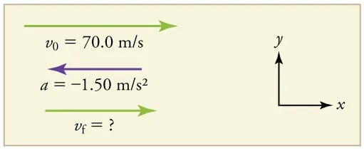
Figure 2.27 Image from OpenStax College Physics 2e, CC-BY 4.0
Image Description
The image is a diagram illustrating a physics problem involving motion. It contains the following elements:
- A green arrow pointing to the right with the text v0 = 70.0 m/s next to it, indicating the initial velocity of an object is 70.0 meters per second.
- A purple arrow pointing to the left with the text a = -1.50 m/s2 next to it, indicating the acceleration of the object is -1.50 meters per second squared.
- A green arrow pointing to the right with the text vf = ?, indicating the final velocity is unknown.
On the right side of the image, there is a small coordinate system with the axes labeled x for horizontal and y for vertical, both arrows pointing in the positive direction.
Solution
1. Identify the knowns. [latex]v_{0} = \text{70} . \text{0 m}/\text{s}[/latex], [latex]a = - 1 . \text{50 m}/\text{s}^{2}[/latex], [latex]t = \text{40} . 0 \text{s}[/latex].
2. Identify the unknown. In this case, it is final velocity, [latex]v_{f}[/latex].
3. Determine which equation to use. We can calculate the final velocity using the equation [latex]v = v_{0} + \text{at}[/latex].
4. Plug in the known values and solve.
[latex]\begin{align*}v &= v_{0} + \text{at}\\ &= \text{70} . \text{0 m}/\text{s} + \left(- 1 . \text{50 m}/\text{s}^{2}\right) \left(\text{40} . \text{0 s}\right)\\ &= \text{10} . \text{0 m}/\text{s}\end{align*}[/latex]
Discussion
The final velocity is much less than the initial velocity, as desired when slowing down, but still positive. With jet engines, reverse thrust could be maintained long enough to stop the plane and start moving it backward. That would be indicated by a negative final velocity, which is not the case here.
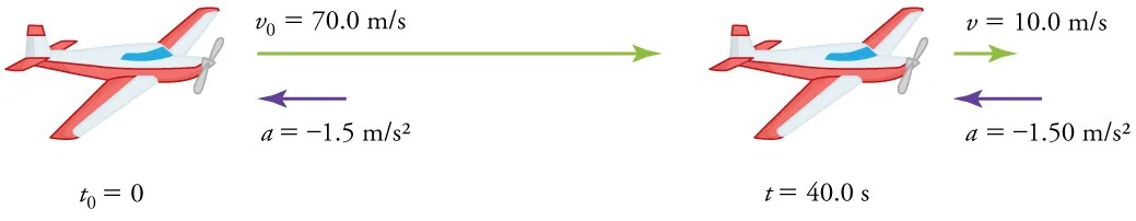
Figure 2.28 The airplane lands with an initial velocity of 70.0 m/s and slows to a final velocity of 10.0 m/s before heading for the terminal. Note that the acceleration is negative because its direction is opposite to its velocity, which is positive. Image from OpenStax College Physics 2e, CC-BY 4.0
Image Description
The image depicts two illustrations of an airplane showing its motion with corresponding initial and final velocities, along with acceleration.
– On the left side, the airplane is shown with a label indicating the initial time, t0 = 0. The initial velocity is labeled as v0 = 70.0 m/s, with a green arrow pointing to the right, indicating the direction of motion. A purple arrow is pointing to the left, labeled with an acceleration of a = -1.5 m/s2, indicating deceleration.
– On the right side, the same airplane is shown at a later time, labeled as t = 40.0 s. The final velocity is labeled as v = 10.0 m/s with a green arrow still pointing to the right. A similar purple arrow pointing to the left indicates the same deceleration with a = -1.5 m/s2.
Overall, the illustration demonstrates a decelerating motion of an airplane from a higher initial velocity to a lower final velocity over a specific time period.
In addition to being useful in problem solving, the equation [latex]v = v_{0} + \text{at}[/latex] gives us insight into the relationships among velocity, acceleration, and time. From it we can see, for example, that
- final velocity depends on how large the acceleration is and how long it lasts
- if the acceleration is zero, then the final velocity equals the initial velocity [latex]\left(\right. v = v_{0} \left.\right)[/latex], as expected (i.e., velocity is constant)
- if [latex]a[/latex] is negative, then the final velocity is less than the initial velocity
(All of these observations fit our intuition, and it is always useful to examine basic equations in light of our intuition and experiences to check that they do indeed describe nature accurately.)
Making Connections: Real-World Connection
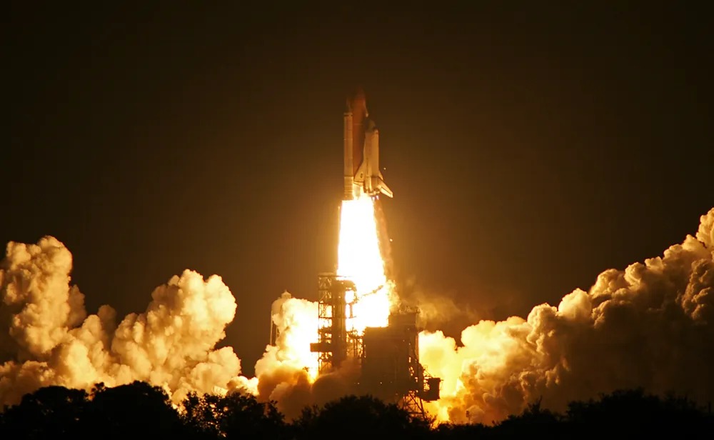
Endeavor
Figure 2.29 The Space Shuttle blasts off from the Kennedy Space Center in February 2010. Image from OpenStax College Physics 2e, CC-BY 4.0
An intercontinental ballistic missile (ICBM) has a larger average acceleration than the Space Shuttle and achieves a greater velocity in the first minute or two of flight (actual ICBM burn times are classified—short-burn-time missiles are more difficult for an enemy to destroy). But the Space Shuttle obtains a greater final velocity, so that it can orbit the earth rather than come directly back down as an ICBM does. The Space Shuttle does this by accelerating for a longer time.
Solving for Final Position When Velocity is Not Constant ([latex]{\color{white}a\neq 0}[/latex])
We can combine the equations above to find a third equation that allows us to calculate the final position of an object experiencing constant acceleration. We start with
[latex]v = v_{0} + \text{at} .[/latex]
Adding [latex]v_{0}[/latex] to each side of this equation and dividing by 2 gives
[latex]\frac{v_{0} + v}{2} = v_{0} + \frac{1}{2} \text{at} .[/latex]
Since [latex]\frac{v_{0} + v}{2} = \overset{-}{v}[/latex] for constant acceleration, then
[latex]\overset{-}{v} = v_{0} + \frac{1}{2} \text{at} .[/latex]
Now we substitute this expression for [latex]\overset{-}{v}[/latex] into the equation for displacement, [latex]x = x_{0} + \overset{-}{v} t[/latex], yielding
[latex]x = x_{0} + v_{0} t + \frac{1}{2} \text{at}^{2} \left(\right. \text{constant } a \left.\right) .[/latex]
Example 2.10
Calculating Displacement of an Accelerating Object: Dragsters
Dragsters can achieve average accelerations of [latex]\text{26} . \text{0 m}/\text{s}^{2}[/latex]. Suppose such a dragster accelerates from rest at this rate for 5.56 s. How far does it travel in this time?
Strategy
Draw a sketch.
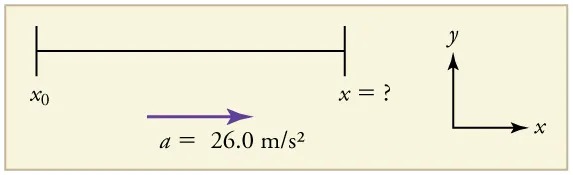
Figure 2.31 Image from OpenStax College Physics 2e, CC-BY 4.0
Image Description
The image illustrates a physics problem involving motion. It includes a horizontal line with two vertical ticks at both ends. The left tick is labeled x0, and the right tick is labeled x = ?. An arrow pointing to the right is positioned below the line, indicating acceleration. The equation a = 26.0 m/s2 is written beside the arrow, specifying the acceleration value. On the right side of the image, a coordinate system is shown with y indicated as the vertical axis and x as the horizontal axis.
We are asked to find displacement, which is [latex]x[/latex] if we take [latex]x_{0}[/latex] to be zero. (Think about it like the starting line of a race. It can be anywhere, but we call it 0 and measure all other positions relative to it.) We can use the equation [latex]x = x_{0} + v_{0} t + \frac{1}{2} \text{at}^{2}[/latex]once we identify [latex]v_{0}[/latex], [latex]a[/latex], and [latex]t[/latex] from the statement of the problem.
Solution
1. Identify the knowns. Starting from rest means that [latex]v_{0} = 0[/latex], [latex]a[/latex] is given as [latex]\text{26} . 0 \text{m}/\text{s}^{2}[/latex] and [latex]t[/latex] is given as 5.56 s.
2. Plug the known values into the equation to solve for the unknown [latex]x[/latex]:
[latex]x = x_{0} + v_{0} t + \frac{1}{2} \text{at}^{2} .[/latex]
Since the initial position and velocity are both zero, this simplifies to
[latex]x = \frac{1}{2} \text{at}^{2} .[/latex]
Substituting the identified values of [latex]a[/latex] and [latex]t[/latex] gives
[latex]x = \frac{1}{2} \left(\text{26} . \text{0 m}/\text{s}^{2}\right) \left(5 . \text{56 s}\right)^{2} ,[/latex]
yielding
[latex]x = \text{402 m}.[/latex]
Discussion
If we convert 402 m to miles, we find that the distance covered is very close to one quarter of a mile, the standard distance for drag racing. So the answer is reasonable. This is an impressive displacement in only 5.56 s, but top-notch dragsters can do a quarter mile in even less time than this.
What else can we learn by examining the equation [latex]x = x_{0} + v_{0} t + \frac{1}{2} \text{at}^{2} ?[/latex] We see that:
- displacement depends on the square of the elapsed time when acceleration is not zero. In Example 2.10, the dragster covers only one fourth of the total distance in the first half of the elapsed time
- if acceleration is zero, then the initial velocity equals average velocity ([latex]v_{0} = \overset{-}{v}[/latex]) and [latex]x = x_{0} + v_{0} t + \frac{1}{2} \text{at}^{2}[/latex] becomes [latex]x = x_{0} + v_{0} t[/latex]
Solving for Final Velocity when Velocity Is Not Constant ([latex]{\color{white}a\neq0}[/latex])
A fourth useful equation can be obtained from another algebraic manipulation of previous equations.
If we solve [latex]v = v_{0} + \text{at}[/latex] for [latex]t[/latex], we get
[latex]t = \frac{v - v_{0}}{a} .[/latex]
Substituting this and [latex]\overset{-}{v} = \frac{v_{0} + v}{2}[/latex] into [latex]x = x_{0} + \overset{-}{v} t[/latex], we get
[latex]v^{2} = v_{0}^{2} + 2 a \left(x - x_{0}\right) \left(\right. \text{constant} a \left.\right) .[/latex]
Example 2.11
Calculating Final Velocity: Dragsters
Calculate the final velocity of the dragster in Example 2.10 without using information about time.
Strategy
Draw a sketch.
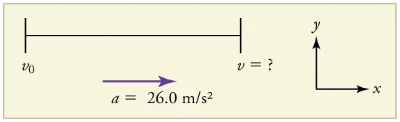
Figure 2.32 Image from OpenStax College Physics 2e, CC-BY 4.0
Image Description
The image contains a physics diagram showing an object’s motion. On the left, there’s an initial velocity denoted as \(v_0\), represented with a short vertical line. To its right, there’s a longer horizontal line ending with another vertical line, indicating the final velocity \(v\), which is unknown. Below the horizontal line, there’s an arrow pointing to the right, labeled with the acceleration \(a = 26.0 \, \text{m/s}^2\). On the right side of the image, there is a set of axes with “x” labeled on the horizontal axis and “y” on the vertical axis. The background is light-colored.
The equation [latex]v^{2} = v_{0}^{2} + 2 a \left(\right. x - x_{0} \left.\right)[/latex] is ideally suited to this task because it relates velocities, acceleration, and displacement, and no time information is required.
Solution
1. Identify the known values. We know that [latex]v_{0} = 0[/latex], since the dragster starts from rest. Then we note that [latex]x - x_{0} = \text{402 m}[/latex] (this was the answer in Example 2.10). Finally, the average acceleration was given to be [latex]a = \text{26} . \text{0 m}/\text{s}^{2}[/latex].
2. Plug the knowns into the equation [latex]v^{2} = v_{0}^{2} + 2 a \left(\right. x - x_{0} \left.\right)[/latex] and solve for [latex]v .[/latex]
[latex]v^{2} = 0 + 2 \left(\text{26} . \text{0 m}/\text{s}^{2}\right) \left(\text{402 m}\right) .[/latex]
Thus
[latex]v^{2} = 2 . \text{09} \times \text{10}^{4} \text{m}^{2} /\text{s}^{2} .[/latex]
To get [latex]v[/latex], we take the square root:
[latex]v = \sqrt{2 . \text{09} \times \text{10}^{4} \text{ m}^{2} /\text{s}^{2}} = \text{145 m}/\text{s} .[/latex]
Discussion
145 m/s is about 522 km/h or about 324 mi/h, but even this breakneck speed is short of the record for the quarter mile. Also, note that a square root has two values; we took the positive value to indicate a velocity in the same direction as the acceleration.
An examination of the equation [latex]v^{2} = v_{0}^{2} + 2 a \left(\right. x - x_{0} \left.\right)[/latex] can produce further insights into the general relationships among physical quantities:
- The final velocity depends on how large the acceleration is and the distance over which it acts
- For a fixed deceleration, a car that is going twice as fast doesn’t simply stop in twice the distance—it takes much further to stop. (This is why we have reduced speed zones near schools.)
Putting Equations Together
In the following examples, we further explore one-dimensional motion, but in situations requiring slightly more algebraic manipulation. The examples also give insight into problem-solving techniques. The box below provides easy reference to the equations needed.
Summary of Kinematic Equations (constant [latex]{\color{white}a}[/latex])
[latex]x = x_{0} + \overset{-}{v} t[/latex]
[latex]\overset{-}{v} = \frac{v_{0} + v}{2}[/latex]
[latex]v = v_{0} + \text{at}[/latex]
[latex]x = x_{0} + v_{0} t + \frac{1}{2} \text{at}^{2}[/latex]
[latex]v^{2} = v_{0}^{2} + 2 a \left(x - x_{0}\right)[/latex]
Example 2.12
Calculating Displacement: How Far Does a Car Go When Coming to a Halt?
On dry concrete, a car can decelerate at a rate of [latex]7 . \text{00 m}/\text{s}^{2}[/latex], whereas on wet concrete it can decelerate at only [latex]5 . \text{00 m}/\text{s}^{2}[/latex]. Find the distances necessary to stop a car moving at 30.0 m/s (about 110 km/h) (a) on dry concrete and (b) on wet concrete. (c) Repeat both calculations, finding the displacement from the point where the driver sees a traffic light turn red, taking into account his reaction time of 0.500 s to get his foot on the brake.
Strategy
Draw a sketch.
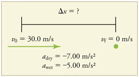
Figure 2.33 Image from OpenStax College Physics 2e, CC-BY 4.0
Image Description
The image depicts a physics problem involving motion and acceleration. It shows an object with initial velocity and final velocity, asking for the displacement (Δx).
The elements in the image are as follows:
- Initial velocity (v0) is 30.0 m/s.
- Final velocity (vf) is 0 m/s.
- Acceleration on dry surface (adry) is -7.00 m/s².
- Acceleration on wet surface (awet) is -5.00 m/s².
There is an arrow pointing leftward, indicating the direction of motion, aligned with the initial velocity.
In order to determine which equations are best to use, we need to list all of the known values and identify exactly what we need to solve for. We shall do this explicitly in the next several examples, using tables to set them off.
Solution for (a)
1. Identify the knowns and what we want to solve for. We know that [latex]v_{0} = \text{30} . \text{0 m}/\text{s}[/latex]; [latex]v = \text{0 }[/latex]; [latex]a = - 7 . \text{00} \text{m}/\text{s}^{2}[/latex] ([latex]a[/latex] is negative because it is in a direction opposite to velocity). We take [latex]x_{0}[/latex] to be 0. We are looking for displacement [latex]Δ x[/latex], or [latex]x - x_{0}[/latex].
2. Identify the equation that will help up solve the problem. The best equation to use is
[latex]v^{2} = v_{0}^{2} + 2 a \left(x - x_{0}\right) .[/latex]
This equation is best because it includes only one unknown, [latex]x[/latex]. We know the values of all the other variables in this equation. (There are other equations that would allow us to solve for [latex]x[/latex], but they require us to know the stopping time, [latex]t[/latex], which we do not know. We could use them but it would entail additional calculations.)
3. Rearrange the equation to solve for [latex]x[/latex].
[latex]x - x_{0} = \frac{v^{2} - v_{0}^{2}}{2 a}[/latex]
4. Enter known values.
[latex]x - 0 = \frac{0^{2} - \left(\text{30} . \text{0 m}/\text{s}\right)^{2}}{2 \left(- 7 . \text{00 m}/\text{s}^{2}\right)}[/latex]
Thus,
[latex]x = \text{64} . \text{3 m on dry concrete} .[/latex]
Solution for (b)
This part can be solved in exactly the same manner as Part A. The only difference is that the deceleration is [latex]– 5 . \text{00 m}/\text{s}^{2}[/latex]. The result is
[latex]x_{\text{wet}} = \text{90} . \text{0 m on wet concrete} .[/latex]
Solution for (c)
Once the driver reacts, the stopping distance is the same as it is in Parts A and B for dry and wet concrete. So to answer this question, we need to calculate how far the car travels during the reaction time, and then add that to the stopping time. It is reasonable to assume that the velocity remains constant during the driver’s reaction time.
1. Identify the knowns and what we want to solve for. We know that [latex]\overset{-}{v} = \text{30}.\text{0 m}/\text{s}[/latex];
[latex]t_{\text{reaction}} = 0.500 \text{s}[/latex];
[latex]a_{\text{reaction}} = 0[/latex]. We take
[latex]x_{0 - \text{reaction}}[/latex] to be 0. We are looking for
[latex]x_{\text{reaction}}[/latex].
2. Identify the best equation to use.
[latex]x = x_{0} + \overset{-}{v} t[/latex] works well because the only unknown value is [latex]x[/latex], which is what we want to solve for.
3. Plug in the knowns to solve the equation.
[latex]x = 0 + \left(\text{30} . \text{0 m}/\text{s}\right) \left(0 . \text{500 s}\right) = \text{15} . \text{0 m} .[/latex]
This means the car travels 15.0 m while the driver reacts, making the total displacements in the two cases of dry and wet concrete 15.0 m greater than if he reacted instantly.
4. Add the displacement during the reaction time to the displacement when braking.
[latex]x_{\text{braking}} + x_{\text{reaction}} = x_{\text{total}}[/latex]
- 64.3 m + 15.0 m = 79.3 m when dry
- 90.0 m + 15.0 m = 105 m when wet
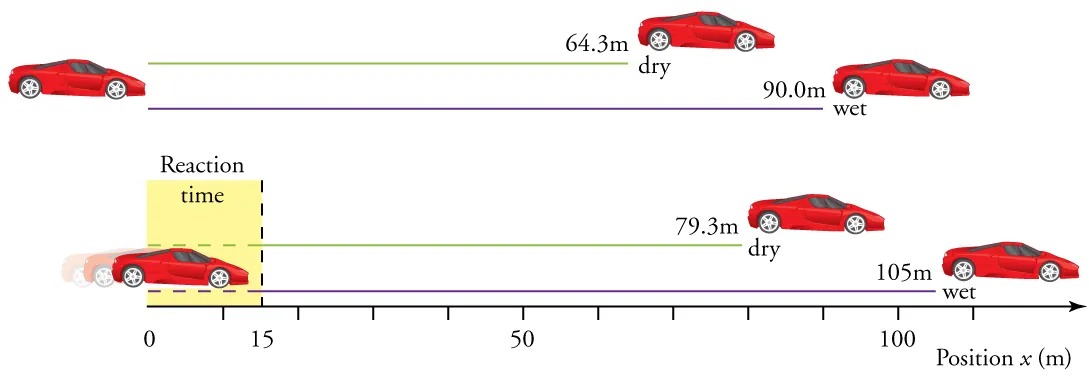
Figure 2.34 The distance necessary to stop a car varies greatly, depending on road conditions and driver reaction time. Shown here are the braking distances for dry and wet pavement, as calculated in this example, for a car initially traveling at 30.0 m/s. Also shown are the total distances traveled from the point where the driver first sees a light turn red, assuming a 0.500 s reaction time. Image from OpenStax College Physics 2e, CC-BY 4.0
Image Description
The image is an illustration showing the stopping distances of a red sports car on dry and wet roads. It depicts two scenarios with labeled stopping distances in meters.
In the upper part of the image:
- Stops at 64.3 meters on a dry road.
- Stops at 90.0 meters on a wet road.
In the lower part of the image:
- Stops at 79.3 meters on a dry road.
- Stops at 105 meters on a wet road.
The bottom of the image shows an axis marked as “Position x (m)” ranging from 0 to 100 meters. There is also a section labeled “Reaction time” at the start, depicted with a yellow box next to a transparent red car moving forward to a solid image of the car at the beginning of the measurement line.
Discussion
The displacements found in this example seem reasonable for stopping a fast-moving car. It should take longer to stop a car on wet rather than dry pavement. It is interesting that reaction time adds significantly to the displacements. But more important is the general approach to solving problems. We identify the knowns and the quantities to be determined and then find an appropriate equation. There is often more than one way to solve a problem. The various parts of this example can in fact be solved by other methods, but the solutions presented above are the shortest.
Example 2.13
Calculating Time: A Car Merges into Traffic
Suppose a car merges into freeway traffic on a 200-m-long ramp. If its initial velocity is 10.0 m/s and it accelerates at [latex]2 . \text{00 m}/\text{s}^{2}[/latex], how long does it take to travel the 200 m up the ramp? (Such information might be useful to a traffic engineer.)
Strategy
Draw a sketch.
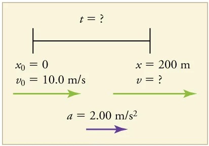
Figure 2.35 Image from OpenStax College Physics 2e, CC-BY 4.0
Image Description
The image is a physics problem illustration involving motion. It is set against a light beige background and includes several equations and annotations:
– At the top center, there is a horizontal line bracket labeled with “t = ?” to indicate that the time is unknown.
– On the left side of the line, it is labeled with:
– \( x_0 = 0 \)
– \( v_0 = 10.0 \, \text{m/s} \)
– This section also features a green arrow pointing to the right, symbolizing initial velocity.
– On the right side, it is labeled with:
– \( x = 200 \, \text{m} \)
– \( v = ? \)
– This portion also has a green arrow pointing to the right, depicting motion towards the final position.
– Centered below the line is the acceleration given by:
– \( a = 2.00 \, \text{m/s}^2 \)
– An accompanying purple arrow pointing to the right illustrates the direction of acceleration.
The problem is asking to determine the unknown final velocity (\( v \)) and the time (\( t \)) while the object moves from position \( x_0 \) to position \( x \) under constant acceleration.
We are asked to solve for the time [latex]t[/latex]. As before, we identify the known quantities in order to choose a convenient physical relationship (that is, an equation with one unknown, [latex]t[/latex]).
Solution
1. Identify the knowns and what we want to solve for. We know that [latex]v_{0} = \text{10 m}/\text{s}[/latex]; [latex]a = 2 . \text{00 m}/\text{s}^{2}[/latex]; and [latex]x = \text{200 m}[/latex].
2. We need to solve for [latex]t[/latex]. Choose the best equation. [latex]x = x_{0} + v_{0} t + \frac{1}{2} \text{at}^{2}[/latex] works best because the only unknown in the equation is the variable [latex]t[/latex] for which we need to solve.
3. We will need to rearrange the equation to solve for [latex]t[/latex]. In this case, it will be easier to plug in the knowns first.
[latex]\text{200 m} = \text{0 m} + \left(\text{10} . \text{0 m}/\text{s}\right) t + \frac{1}{2} \left(2 . \text{00 m}/\text{s}^{2}\right) t^{2}[/latex]
4. Simplify the equation. The units of meters (m) cancel because they are in each term. We can get the units of seconds (s) to cancel by taking [latex]t = t \text{s}[/latex], where [latex]t[/latex] is the magnitude of time and s is the unit. Doing so leaves
[latex]\text{200} = \text{10} t + t^{2} .[/latex]
5. Use the quadratic formula to solve for [latex]t[/latex].
(a) Rearrange the equation to get 0 on one side of the equation.
[latex]t^{2} + \text{10} t - \text{200} = 0[/latex]
This is a quadratic equation of the form
[latex]\text{at}^{2} + \text{bt} + c = 0 ,[/latex]
where the constants are [latex]a = 1 . \text{00}, b = \text{10} . \text{0}, \text{and} c = - \text{200}[/latex].
(b) Its solutions are given by the quadratic formula:
[latex]t = \frac{- b \pm \sqrt{b^{2} - 4 \text{ac}}}{2 a} .[/latex]
This yields two solutions for [latex]t[/latex], which are
[latex]t = \text{10} . 0 \text{and} - \text{20} . 0 .[/latex]
In this case, then, the time is [latex]t = t[/latex] in seconds, or
[latex]t = \text{10} . 0 \text{s} \text{and} - \text{20} . 0 \text{s} .[/latex]
A negative value for time is unreasonable, since it would mean that the event happened 20 s before the motion began. We can discard that solution. Thus,
[latex]t = \text{10} . 0 \text{s} .[/latex]
Discussion
Whenever an equation contains an unknown squared, there will be two solutions. In some problems both solutions are meaningful, but in others, such as the above, only one solution is reasonable. The 10.0 s answer seems reasonable for a typical freeway on-ramp.
With the basics of kinematics established, we can go on to many other interesting examples and applications. In the process of developing kinematics, we have also glimpsed a general approach to problem solving that produces both correct answers and insights into physical relationships. Problem-Solving Basics discusses problem-solving basics and outlines an approach that will help you succeed in this invaluable task.
Making Connections: Take-Home Experiment—Breaking News
We have been using SI units of meters per second squared to describe some examples of acceleration or deceleration of cars, runners, and trains. To achieve a better feel for these numbers, one can measure the braking deceleration of a car doing a slow (and safe) stop. Recall that, for average acceleration, [latex]\overset{-}{a} = Δ v / Δ t[/latex]. While traveling in a car, slowly apply the brakes as you come up to a stop sign. Have a passenger note the initial speed in miles per hour and the time taken (in seconds) to stop. From this, calculate the deceleration in miles per hour per second. Convert this to meters per second squared and compare with other decelerations mentioned in this chapter. Calculate the distance traveled in braking.
Check Your Understanding
A rocket accelerates at a rate of [latex]\text{20 m}/\text{s}^{2}[/latex] during launch. How long does it take the rocket to reach a velocity of 400 m/s?
Click for Solution
Solution
To answer this, choose an equation that allows you to solve for time [latex]t[/latex], given only [latex]a[/latex], [latex]v_{0}[/latex], and [latex]v[/latex].
[latex]v = v_{0} + \text{at}[/latex]
Rearrange to solve for [latex]t[/latex].
[latex]t = \frac{v - v \_{0}^{}}{a} = \frac{\text{400 m}/\text{s} - \text{0 m}/\text{s}}{\text{20 m}/\text{s}^{2}} = \text{20 s}[/latex]
