2.4 Acceleration
Learning Objectives
By the end of this section, you will be able to:
- Define and distinguish between instantaneous acceleration, average acceleration, and deceleration.
- Calculate acceleration given initial time, initial velocity, final time, and final velocity.

Figure 2.12A plane decelerates, or slows down, as it comes in for landing in St. Maarten. Its acceleration is opposite in direction to its velocity. Image from OpenStax College Physics 2e, CC-BY 4.0
In everyday conversation, to accelerate means to speed up. The accelerator in a car can in fact cause it to speed up. The greater the acceleration, the greater the change in velocity over a given time. The formal definition of acceleration is consistent with these notions, but more inclusive.
Average Acceleration
Average Acceleration is the rate at which velocity changes,
[latex]\overset{-}{a} = \frac{Δ v}{Δ t} = \frac{v_{f} - v_{0}}{t_{f} - t_{0}} ,[/latex]
where [latex]\overset{-}{a}[/latex] is average acceleration, [latex]v[/latex] is velocity, and [latex]t[/latex] is time. (The bar over the [latex]a[/latex] means average acceleration.)
Because acceleration is velocity in m/s divided by time in s, the SI units for acceleration are [latex]\text{m}/\text{s}^{2}[/latex], meters per second squared or meters per second per second, which literally means by how many meters per second the velocity changes every second.
Recall that velocity is a vector—it has both magnitude and direction. This means that a change in velocity can be a change in magnitude (or speed), but it can also be a change in direction. For example, if a car turns a corner at constant speed, it is accelerating because its direction is changing. The quicker you turn, the greater the acceleration. So there is an acceleration when velocity changes either in magnitude (an increase or decrease in speed) or in direction, or both.
Acceleration as a Vector
Acceleration is a vector in the same direction as the change in velocity, [latex]Δ v[/latex]. Since velocity is a vector, it can change either in magnitude or in direction. Acceleration is therefore a change in either speed or direction, or both.
Keep in mind that although acceleration is in the direction of the change in velocity, it is not always in the direction of motion. When an object slows down, its acceleration is opposite to the direction of its motion. This is known as deceleration.
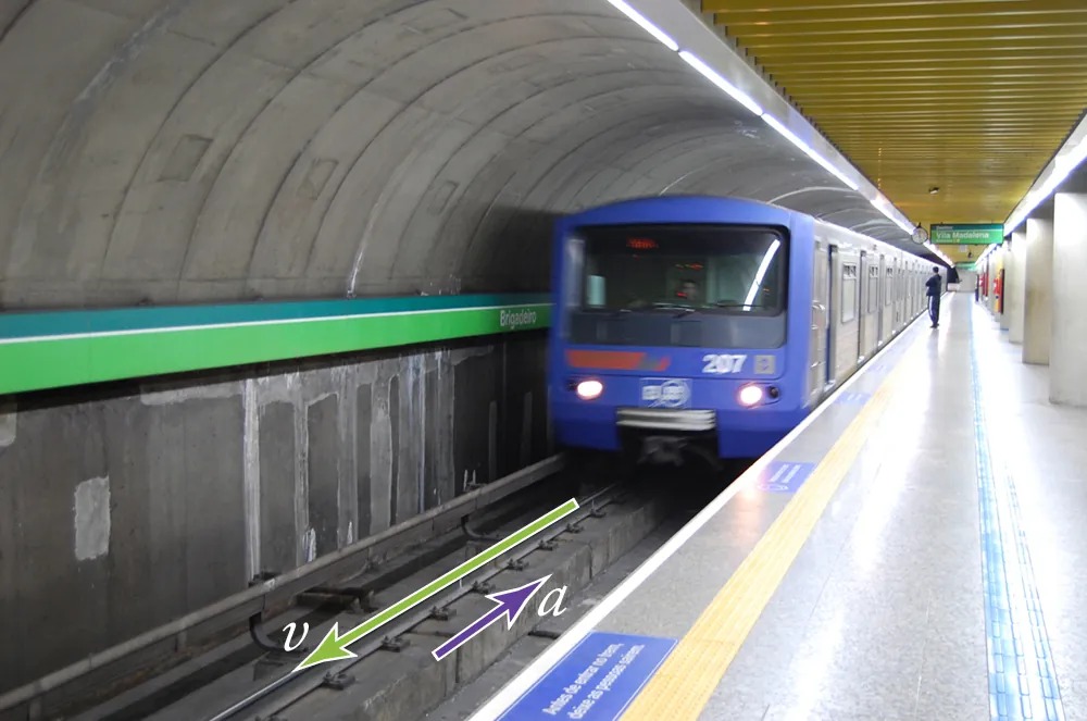
Figure 2.13 A subway train in Sao Paulo, Brazil, decelerates as it comes into a station. It is accelerating in a direction opposite to its direction of motion. Image from OpenStax College Physics 2e, CC-BY 4.0
Misconception Alert: Deceleration vs. Negative Acceleration
Deceleration always refers to acceleration in the direction opposite to the direction of the velocity. Deceleration always reduces speed. Negative acceleration, however, is acceleration in the negative direction in the chosen coordinate system. Negative acceleration may or may not be deceleration, and deceleration may or may not be considered negative acceleration. For example, consider Figure 2.14.

Figure 2.14(a) This car is speeding up as it moves toward the right. It therefore has positive acceleration in our coordinate system. (b) This car is slowing down as it moves toward the right. Therefore, it has negative acceleration in our coordinate system, because its acceleration is toward the left. The car is also decelerating: the direction of its acceleration is opposite to its direction of motion. (c) This car is moving toward the left, but slowing down over time. Therefore, its acceleration is positive in our coordinate system because it is toward the right. However, the car is decelerating because its acceleration is opposite to its motion. (d) This car is speeding up as it moves toward the left. It has negative acceleration because it is accelerating toward the left. However, because its acceleration is in the same direction as its motion, it is speeding up (not decelerating) Image from OpenStax College Physics 2e, CC-BY 4.0
Example 2.1
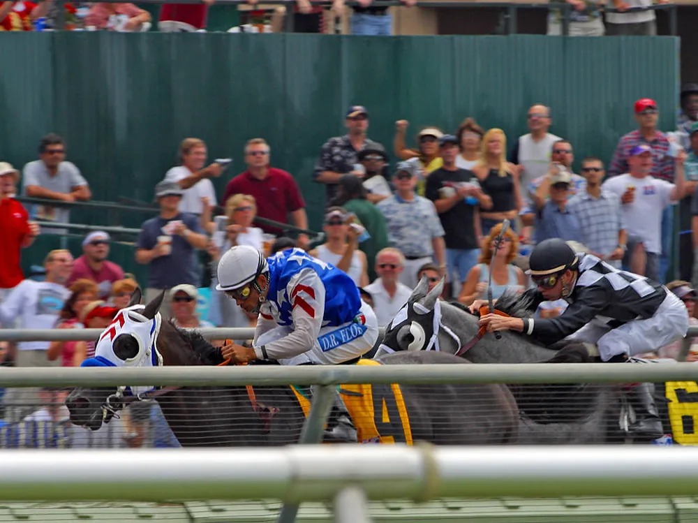
Calculating Acceleration: A Racehorse Leaves the Gate
A racehorse coming out of the gate accelerates from rest to a velocity of 15.0 m/s due west in 1.80 s. What is its average acceleration?
Strategy
First we draw a sketch and assign a coordinate system to the problem. This is a simple problem, but it always helps to visualize it. Notice that we assign east as positive and west as negative. Thus, in this case, we have negative velocity.
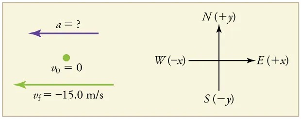
Figure 2.16 Image from OpenStax College Physics 2e, CC-BY 4.0
Image Description
The image is divided into two sections.
Left Section:
– There is a horizontal arrow pointing to the left, labeled with a purple label: “a = ?” This indicates an unknown acceleration directed to the left.
– Below this, there is a green dot with the label “v₀ = 0,” indicating an initial velocity of zero.
– Beneath the dot, another horizontal arrow points to the left, labeled with a green label: “vₒ = -15.0 m/s,” indicating a final velocity of -15.0 meters per second.
Right Section:
– A coordinate system is shown with four arrows:
– “N (+y)” indicates an upward direction (positive y-axis).
– “E (+x)” indicates a rightward direction (positive x-axis).
– “S (-y)” indicates a downward direction (negative y-axis).
– “W (-x)” indicates a leftward direction (negative x-axis).
We can solve this problem by identifying [latex]Δ v[/latex] and [latex]Δ t[/latex] from the given information and then calculating the average acceleration directly from the equation [latex]\overset{-}{a} = \frac{Δ v}{Δ t} = \frac{v_{f} - v_{0}}{t_{f} - t_{0}}[/latex].
Solution
1. Identify the knowns. [latex]v_{0} = 0[/latex], [latex]v_{f} = - \text{15} .\text{0 m}/\text{s}[/latex] (the negative sign indicates direction toward the west), [latex]Δ t = 1 .\text{80 s}[/latex].
2. Find the change in velocity. Since the horse is going from zero to [latex]- \text{15}.\text{0 m}/\text{s}[/latex], its change in velocity equals its final velocity: [latex]Δ v = v_{f} = - \text{15} .\text{0 m}/\text{s}[/latex].
3. Plug in the known values ([latex]Δ v[/latex] and [latex]Δ t[/latex]) and solve for the unknown [latex]\overset{-}{a}[/latex].
[latex]\overset{-}{a} = \frac{Δ v}{Δ t} = \frac{- \text{15} .\text{0 m}/\text{s }}{1 .\text{80 s}} = - 8 .\text{33 m} /\text{s}^{2} .[/latex]
Discussion
The negative sign for acceleration indicates that acceleration is toward the west. An acceleration of [latex]8 .\text{33 m} /\text{s}^{2}[/latex] due west means that the horse increases its velocity by 8.33 m/s due west each second, that is, 8.33 meters per second per second, which we write as [latex]8 .\text{33 m} /\text{s}^{2}[/latex]. This is truly an average acceleration, because the ride is not smooth. We shall see later that an acceleration of this magnitude would require the rider to hang on with a force nearly equal to his weight.
Instantaneous Acceleration
Instantaneous acceleration [latex]a[/latex], or the acceleration at a specific instant in time, is obtained by the same process as discussed for instantaneous velocity in 2.3 Time, Velocity, and Speed—that is, by considering an infinitesimally small interval of time. How do we find instantaneous acceleration using only algebra? The answer is that we choose an average acceleration that is representative of the motion. Figure 2.17 shows graphs of instantaneous acceleration versus time for two very different motions. In Figure 2.17(a), the acceleration varies slightly and the average over the entire interval is nearly the same as the instantaneous acceleration at any time. In this case, we should treat this motion as if it had a constant acceleration equal to the average (in this case about [latex]1 . 8 m /\text{s}^{2}[/latex]). In Figure 2.17(b), the acceleration varies drastically over time. In such situations it is best to consider smaller time intervals and choose an average acceleration for each. For example, we could consider motion over the time intervals from 0 to 1.0 s and from 1.0 to 3.0 s as separate motions with accelerations of [latex]+ 3 . 0 m /\text{s}^{2}[/latex] and [latex]–\text{2} . 0 m /\text{s}^{2}[/latex], respectively.
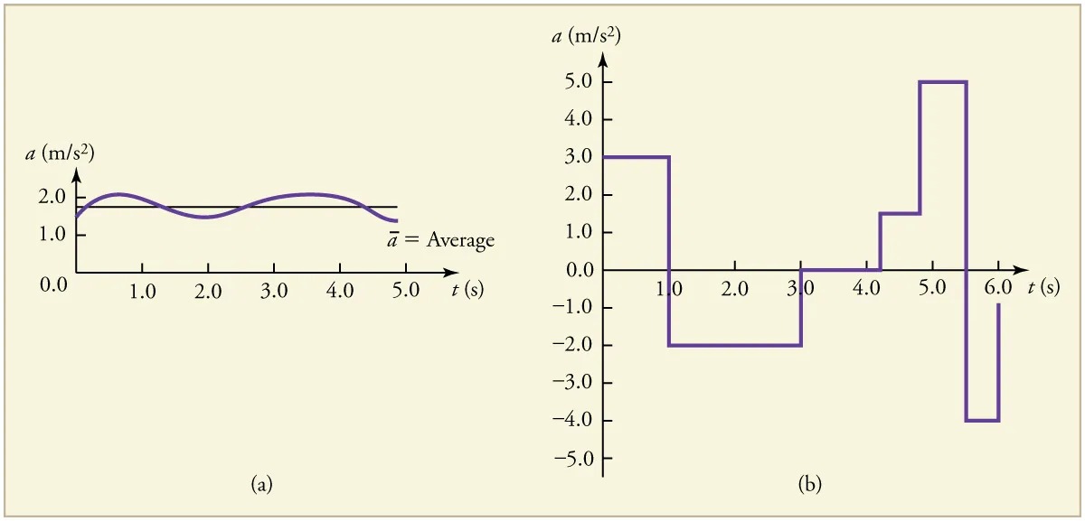
Figure 2.17Graphs of instantaneous acceleration versus time for two different one-dimensional motions. (a) Here acceleration varies only slightly and is always in the same direction, since it is positive. The average over the interval is nearly the same as the acceleration at any given time. (b) Here the acceleration varies greatly, perhaps representing a package on a post office conveyor belt that is accelerated forward and backward as it bumps along. It is necessary to consider small time intervals (such as from 0 to 1.0 s) with constant or nearly constant acceleration in such a situation. Image from OpenStax College Physics 2e, CC-BY 4.0
Image Description
The image consists of two graphs labeled (a) and (b), side by side.
Graph (a):
– Axis Labels: The vertical axis is labeled as “a (m/s²)” representing acceleration in meters per second squared. The horizontal axis is labeled as “t (s)” representing time in seconds.
– Data Representation: The graph shows a sinusoidal wave fluctuating around a horizontal line labeled “a̅ = Average.” The wave oscillates between approximately 0 and 2 m/s² over 6 seconds.
– Average Line: A horizontal line indicating the average value, running at approximately 1.0 m/s².
Graph (b):
– Axis Labels: Similar to graph (a), the vertical axis is labeled “a (m/s²)” and the horizontal axis is labeled “t (s).”
– Data Representation: This graph features a step function with varying values of acceleration over time:
– From 0 to 1 second, the acceleration is 3 m/s².
– From 1 to 3 seconds, the acceleration drops to -3 m/s².
– From 3 to 4 seconds, the acceleration is 0 m/s².
– From 4 to 5 seconds, the acceleration increases to 2 m/s².
– From 5 to 6 seconds, the acceleration is -5 m/s².
Both graphs depict acceleration versus time relationships but in different forms; one is a smooth wave, and the other is a series of steps.
The next several examples consider the motion of the subway train shown in Figure 2.18. In (a) the shuttle moves to the right, and in (b) it moves to the left. The examples are designed to further illustrate aspects of motion and to illustrate some of the reasoning that goes into solving problems.
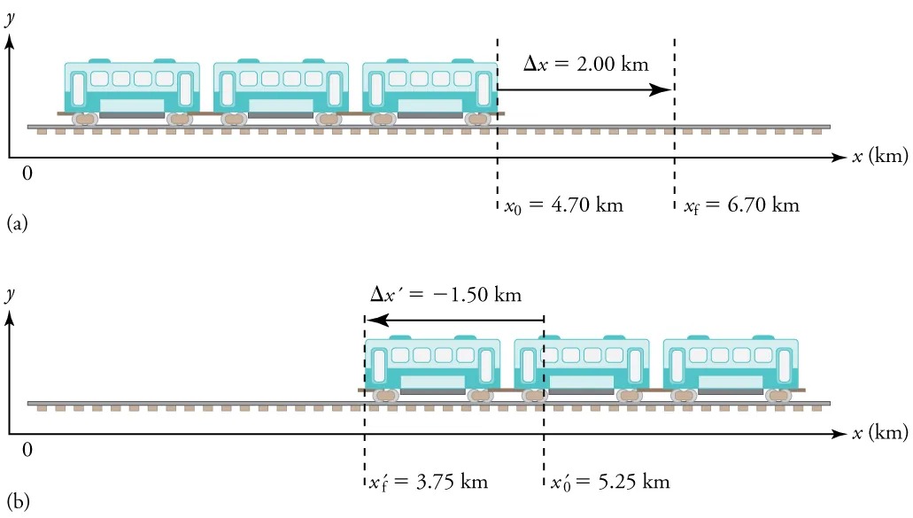
Figure 2.18One-dimensional motion of a subway train considered in , , , , , and . Here we have chosen the [latex]x[/latex]-axis so that + means to the right and [latex]-[/latex] means to the left for displacements, velocities, and accelerations. (a) The subway train moves to the right from [latex]x_{0}[/latex] to[latex]x_{f}[/latex]. Its displacement[latex]Δ x[/latex] is +2.0 km. (b) The train moves to the left from[latex]\left(x '\right)_{0}[/latex] to[latex]\left(x '\right)_{f}[/latex]. Its displacement [latex]Δ x '[/latex] is [latex]- 1 .\text{5 km}[/latex]. Image from OpenStax College Physics 2e, CC-BY 4.0
Example 2.2
Calculating Displacement: A Subway Train
What are the magnitude and sign of displacements for the motions of the subway train shown in parts (a) and (b) of Figure 2.18?
Strategy
A drawing with a coordinate system is already provided, so we don’t need to make a sketch, but we should analyze it to make sure we understand what it is showing. Pay particular attention to the coordinate system. To find displacement, we use the equation [latex]Δ x = x_{f} - x_{0}[/latex]. This is straightforward since the initial and final positions are given.
Solution
1. Identify the knowns. In the figure we see that [latex]x_{f} = \text{6}.\text{70 km}[/latex] and
[latex]x_{0} = \text{4}.\text{70 km}[/latex] for part (a), and [latex]\left(x '\right)_{f} = 3 .\text{75 km}[/latex] and [latex]\left(x '\right)_{0} = 5 .\text{25 km}[/latex] for part (b).
2. Solve for displacement in part (a).
[latex]\begin{align*}Δ x& = x_{f} - x_{0}\\ &= 6 . \text{70 km} - 4 . \text{70 km} \\ &= + 2 . \text{00 km}\end{align*}[/latex]
3. Solve for displacement in part (b).
[latex]\begin{align*}Δ x ' &= \left(x '\right)_{f} - \left(x '\right)_{0}\\ &= \text{3}.\text{75 km} - \text{5}.\text{25 km}\\ &= - \text{1}.\text{50 km}\end{align*}[/latex]
Discussion
The direction of the motion in (a) is to the right and therefore its displacement has a positive sign, whereas motion in (b) is to the left and thus has a negative sign.
Example 2.3
Comparing Distance Traveled with Displacement: A Subway Train
What are the distances traveled for the motions shown in parts (a) and (b) of the subway train in Figure 2.18?
Strategy
To answer this question, think about the definitions of distance and distance traveled, and how they are related to displacement. Distance between two positions is defined to be the magnitude of displacement, which was found in Example 2.2. Distance traveled is the total length of the path traveled between the two positions. (See 2.1 Displacement.) In the case of the subway train shown in Figure 2.18, the distance traveled is the same as the distance between the initial and final positions of the train.
Solution
1. The displacement for part (a) was +2.00 km. Therefore, the distance between the initial and final positions was 2.00 km, and the distance traveled was 2.00 km.
2. The displacement for part (b) was [latex]−\text{1}.\text{5 km}.[/latex] Therefore, the distance between the initial and final positions was 1.50 km, and the distance traveled was 1.50 km.
Discussion
Distance is a scalar. It has magnitude but no sign to indicate direction.
Example 2.4
Calculating Acceleration: A Subway Train Speeding Up
Suppose the train in Figure 2.18(a) accelerates from rest to 30.0 km/h in the first 20.0 s of its motion. What is its average acceleration during that time interval?
Strategy
It is worth it at this point to make a simple sketch:
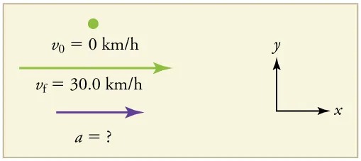
Figure 2.19 Image from OpenStax College Physics 2e, CC-BY 4.0
Image Description
The image depicts a physics problem involving motion. On the left side, there are three expressions:
- v0 = 0 km/h with a green arrow pointing to the right.
- vf = 30.0 km/h with a purple arrow pointing to the right.
- a = ? indicating that acceleration is unknown, represented with a purple arrow.
There is a green dot above the expression for v0.
On the right side, an x-y coordinate system is shown with axes labeled: ‘x’ for the horizontal axis pointing to the right, and ‘y’ for the vertical axis pointing upwards.
This problem involves three steps. First we must determine the change in velocity, then we must determine the change in time, and finally we use these values to calculate the acceleration.
Solution
1. Identify the knowns. [latex]v_{0} = 0[/latex] (the trains starts at rest), [latex]v_{f} = \text{30} . \text{0 km}/\text{h}[/latex], and [latex]Δ t = \text{20} . \text{0 s}[/latex].
2. Calculate [latex]Δ v[/latex]. Since the train starts from rest, its change in velocity is [latex]Δ v = + \text{30}.\text{0 km}/\text{h}[/latex], where the plus sign means velocity to the right.
3. Plug in known values and solve for the unknown, [latex]\overset{-}{a}[/latex].
[latex]\overset{-}{a} = \frac{Δ v}{Δ t} = \frac{+ \text{30}.\text{0 km}/\text{h}}{\text{20} . 0 s}[/latex]
4. Since the units are mixed (we have both hours and seconds for time), we need to convert everything into SI units of meters and seconds. (See 1.2 Physical Quantities and Units for more guidance.)
[latex]\overset{-}{a} = \left(\frac{+ \text{30 km}/\text{h}}{\text{20}.\text{0 s}}\right) \left(\frac{\text{10}^{3} \text{ m}}{\text{1 km}}\right) \left(\frac{\text{1 h}}{\text{3600 s}}\right) = 0 . \text{417 m}/\text{s}^{2}[/latex]
Discussion
The plus sign means that acceleration is to the right. This is reasonable because the train starts from rest and ends up with a velocity to the right (also positive). So acceleration is in the same direction as the change in velocity, as is always the case.
Example 2.5
Calculate Acceleration: A Subway Train Slowing Down
Now suppose that at the end of its trip, the train in Figure 2.18(a) slows to a stop from a speed of 30.0 km/h in 8.00 s. What is its average acceleration while stopping?
Strategy
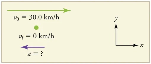
Figure 2.20 Image from OpenStax College Physics 2e, CC-BY 4.0
Image Description
The image features a diagram with the following components:
– On the left side, there is a green horizontal arrow pointing to the right, labeled as v0 = 30.0 km/h. This indicates the initial velocity.
– Below that, a green dot is placed, alongside which is written vf = 0 km/h representing the final velocity.
– Further below, there is a purple horizontal arrow pointing to the left, labeled as a = ?. This suggests an unknown acceleration.
– On the right side of the diagram, there is a set of axes. The y-axis points upwards, and the x-axis points to the right. They are labeled with their respective directions.
The overall background of the image is a soft beige color, framed with a light border.
In this case, the train is decelerating and its acceleration is negative because it is toward the left. As in the previous example, we must find the change in velocity and the change in time and then solve for acceleration.
Solution
1. Identify the knowns. [latex]v_{0} = \text{30} .\text{0 km}/\text{h}[/latex], [latex]v_{f} = 0 km/h[/latex] (the train is stopped, so its velocity is 0), and [latex]Δ t = \text{8}.\text{00 s}[/latex].
2. Solve for the change in velocity, [latex]Δ v[/latex].
[latex]Δ v = v_{f} - v_{0} = 0 - \text{30} . \text{0 km}/\text{h} = - \text{30} .\text{0 km}/\text{h}[/latex]
3. Plug in the knowns, [latex]Δ v[/latex] and [latex]Δ t[/latex], and solve for [latex]\overset{-}{a}[/latex].
[latex]\overset{-}{a} = \frac{Δ v}{Δ t} = \frac{- \text{30} . \text{0 km}/\text{h}}{8 . \text{00 s}}[/latex]
4. Convert the units to meters and seconds.
[latex]\begin{align*}\overset{-}{a} &= \frac{Δ v}{Δ t}\\ &= \left(\frac{- \text{30}.\text{0 km}/\text{h}}{\text{8}.\text{00 s}}\right) \left(\frac{\text{10}^{3} \text{ m}}{\text{1 km}}\right) \left(\frac{\text{1 h}}{\text{3600 s}}\right)\\ &= −\text{1}.\text{04 m}/\text{s}^{2} .\end{align*}[/latex]
Discussion
The minus sign indicates that acceleration is to the left. This sign is reasonable because the train initially has a positive velocity in this problem, and a negative acceleration would oppose the motion. Again, acceleration is in the same direction as the change in velocity, which is negative here. This acceleration can be called a deceleration because it has a direction opposite to the velocity.
The graphs of position, velocity, and acceleration vs. time for the trains in Example 2.4 and Example 2.5 are displayed in Figure 2.21. (We have taken the velocity to remain constant from 20 to 40 s, after which the train decelerates.)
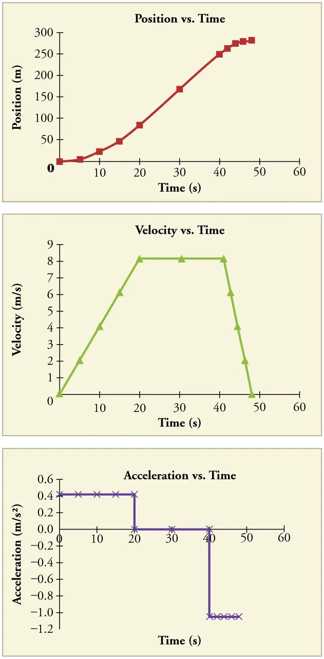
Figure 2.21(a) Position of the train over time. Notice that the train’s position changes slowly at the beginning of the journey, then more and more quickly as it picks up speed. Its position then changes more slowly as it slows down at the end of the journey. In the middle of the journey, while the velocity remains constant, the position changes at a constant rate. (b) Velocity of the train over time. The train’s velocity increases as it accelerates at the beginning of the journey. It remains the same in the middle of the journey (where there is no acceleration). It decreases as the train decelerates at the end of the journey. (c) The acceleration of the train over time. The train has positive acceleration as it speeds up at the beginning of the journey. It has no acceleration as it travels at constant velocity in the middle of the journey. Its acceleration is negative as it slows down at the end of the journey. Image from OpenStax College Physics 2e, CC-BY 4.0
Image Description
The image contains three line graphs stacked vertically, each illustrating different aspects of motion over time.
1. Top Graph: Position vs. Time
– Description: This graph is a plot of position (in meters) against time (in seconds). The graph shows a red line with square markers that starts near the origin (0,0) and curves upwards, indicating an increase in position over time. The line has sections with varying steepness, suggesting changes in speed.
– X-axis: Labeled “Time (s)” and ranges from 0 to 60.
– Y-axis: Labeled “Position (m)” and ranges from 0 to 300.
2. Middle Graph: Velocity vs. Time
– Description: This graph shows velocity (in meters per second) plotted against time. A green line with triangular markers illustrates the velocity starting at zero, increasing to a peak around 5 m/s, remaining steady, and eventually decreasing back to zero.
– X-axis: Labeled “Time (s)” and ranges from 0 to 60.
– Y-axis: Labeled “Velocity (m/s)” and ranges from 0 to 9.
3. Bottom Graph: Acceleration vs. Time
– Description: The graph plots acceleration (in meters per second squared) against time. A purple line with cross markers shows segments of constant acceleration, beginning at 0.4, dropping to zero, and eventually decreasing to -1.0 before stabilizing.
– X-axis: Labeled “Time (s)” and ranges from 0 to 60.
– Y-axis: Labeled “Acceleration (m/s²)” and ranges from -1.2 to 0.6.
Each graph provides a visual representation of different physical quantities describing motion as functions of time.
Example 2.6
Calculating Average Velocity: The Subway Train
What is the average velocity of the train in part b of Example 2.2, and shown again below, if it takes 5.00 min to make its trip?
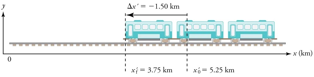
Figure 2.22 Image from OpenStax College Physics 2e, CC-BY 4.0
Image Description
The image depicts a diagram of a train on a straight railway track. The train consists of three connected light blue carriages, and it is shown moving along the track in a negative x-direction.
– Axis Information:
– The horizontal axis is labeled with “x (km)” with an arrow pointing to the right, indicating increasing x-values.
– The vertical axis is labeled with “y” with an upward arrow marked from 0, indicating increasing y-values.
– Train Positioning:
– The train’s motion indicates a change in position from an initial to a final state.
– The initial position of the train is marked at \( x’_0 = 5.25 \) km.
– The final position of the train is marked at \( x’_f = 3.75 \) km.
– The change in position is marked as \( \Delta x’ = -1.50 \) km, indicating a movement backward along the track.
– Additional Details:
– The positions \( x’_0 \) and \( x’_f \) are marked on the track with dashed vertical lines extending upwards to highlight the positions of the train.
The diagram serves to visually represent the displacement of the train along the track over a specific distance.
Strategy
Average velocity is displacement divided by time. It will be negative here, since the train moves to the left and has a negative displacement.
Solution
1. Identify the knowns. [latex]\left(x '\right)_{f} = 3 .\text{75 km}[/latex], [latex]\left(x '\right)_{0} = \text{5}.\text{25 km}[/latex], [latex]Δ t = \text{5}.\text{00 min}[/latex].
2. Determine displacement, [latex]Δ x '[/latex]. We found [latex]Δ x '[/latex] to be [latex]- \text{1}.\text{5 km}[/latex] in Example 2.2.
3. Solve for average velocity.
[latex]\overset{-}{v} = \frac{Δ x '}{Δ t} = \frac{- \text{1}.\text{50 km}}{\text{5}.\text{00 min}}[/latex]
4. Convert units.
[latex]\overset{-}{v} = \frac{Δ x '}{Δ t} = \left(\frac{- 1 . \text{50 km}}{5 . \text{00 min}}\right) \left(\frac{\text{60 min}}{1 h}\right) = - \text{18} .\text{0 km}/\text{h}[/latex]
Discussion
The negative velocity indicates motion to the left.
Example 2.7
Calculating Deceleration: The Subway Train
Finally, suppose the train in Figure 2.22 slows to a stop from a velocity of 20.0 km/h in 10.0 s. What is its average acceleration?
Strategy
Once again, let’s draw a sketch:
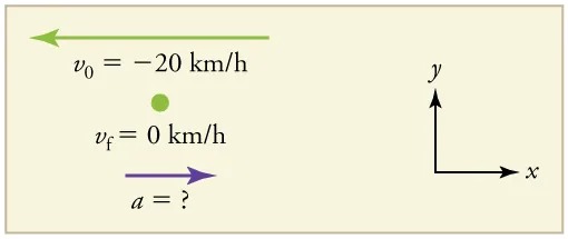
Figure 2.23 Image from OpenStax College Physics 2e, CC-BY 4.0
Image Description
The image consists of the following elements:
– Vectors and Equations:
– A green arrow pointing to the left labeled with the initial velocity equation: \( v_0 = -20 \, \text{km/h} \).
– A point labeled \( v_f = 0 \, \text{km/h} \), indicating the final velocity.
– A purple arrow pointing to the right labeled with the acceleration equation: \( a = ? \).
– Coordinate Axes:
– On the right side, there is a set of coordinate axes. The horizontal axis is labeled as \( x \) and the vertical axis is labeled as \( y \).
As before, we must find the change in velocity and the change in time to calculate average acceleration.
Solution
1. Identify the knowns. [latex]v_{0} = - \text{20}.\text{0 km}/\text{h}[/latex],
[latex]v_{f} = 0 km/h[/latex],
[latex]Δ t = \text{10} . 0 s[/latex].
2. Calculate [latex]Δ v[/latex]. The change in velocity here is actually positive, since
[latex]\begin{align*}Δ v &= v_{f} - v_{0}\\ &= 0 - \left(- \text{20 km}/\text{h}\right)\\ &= + \text{20}.\text{0 km}/\text{h} .\end{align*}[/latex]
3. Solve for [latex]\overset{-}{a}[/latex].
[latex]\overset{-}{a} = \frac{Δ v}{Δ t} = \frac{+ 20.0 \text{km}/\text{h}}{10.0 \text{s}}[/latex]
4. Convert units.
[latex]\begin{align*}\overset{-}{a} &= \left(\frac{+ 20.0 \text{km}/\text{h}}{10.0 \text{s}}\right) \left(\frac{\text{10}^{3} m}{1 km}\right) \left(\frac{1 h}{\text{3600 s}}\right)\\ &= + 0.556 \text{m}/\text{s}^{2}\end{align*}[/latex]
Discussion
The plus sign means that acceleration is to the right. This is reasonable because the train initially has a negative velocity (to the left) in this problem and a positive acceleration opposes the motion (and so it is to the right). Again, acceleration is in the same direction as the change in velocity, which is positive here. As in Example 2.5, this acceleration can be called a deceleration since it is in the direction opposite to the velocity.
Sign and Direction
Perhaps the most important thing to note about these examples is the signs of the answers. In our chosen coordinate system, plus means the quantity is to the right and minus means it is to the left. This is easy to imagine for displacement and velocity. But it is a little less obvious for acceleration. Most people interpret negative acceleration as the slowing of an object. This was not the case in Example 2.7, where a positive acceleration slowed a negative velocity. The crucial distinction was that the acceleration was in the opposite direction from the velocity. In fact, a negative acceleration will increase a negative velocity. For example, the train moving to the left in Figure 2.22 is sped up by an acceleration to the left. In that case, both [latex]v[/latex] and [latex]a[/latex] are negative. The plus and minus signs give the directions of the accelerations. If acceleration has the same sign as the velocity, the object is speeding up. If acceleration has the opposite sign as the velocity, the object is slowing down.
Check Your Understanding
An airplane lands on a runway traveling east. Describe its acceleration.
Click for Solution
Solution
If we take east to be positive, then the airplane has negative acceleration, as it is accelerating toward the west. It is also decelerating: its acceleration is opposite in direction to its velocity.
PhET Explorations
Moving Man Simulation
Learn about position, velocity, and acceleration graphs. Move the little man back and forth with the mouse and plot his motion. Set the position, velocity, or acceleration and let the simulation move the man for you.
