17.6 The Hall Effect
Learning Objectives
By the end of this section, you will be able to:
- Describe the Hall effect.
- Calculate the Hall emf across a current-carrying conductor.
We have seen effects of a magnetic field on free-moving charges. The magnetic field also affects charges moving in a conductor. One result is the Hall effect, which has important implications and applications.
Figure 17.26 shows what happens to charges moving through a conductor in a magnetic field. The field is perpendicular to the electron drift velocity and to the width of the conductor. Note that conventional current is to the right in both parts of the figure. In part (a), electrons carry the current and move to the left. In part (b), positive charges carry the current and move to the right. Moving electrons feel a magnetic force toward one side of the conductor, leaving a net positive charge on the other side. This separation of charge creates a voltage [latex]\epsilon[/latex], known as the Hall emf, across the conductor. The creation of a voltage across a current-carrying conductor by a magnetic field is known as the Hall effect, after Edwin Hall, the American physicist who discovered it in 1879.
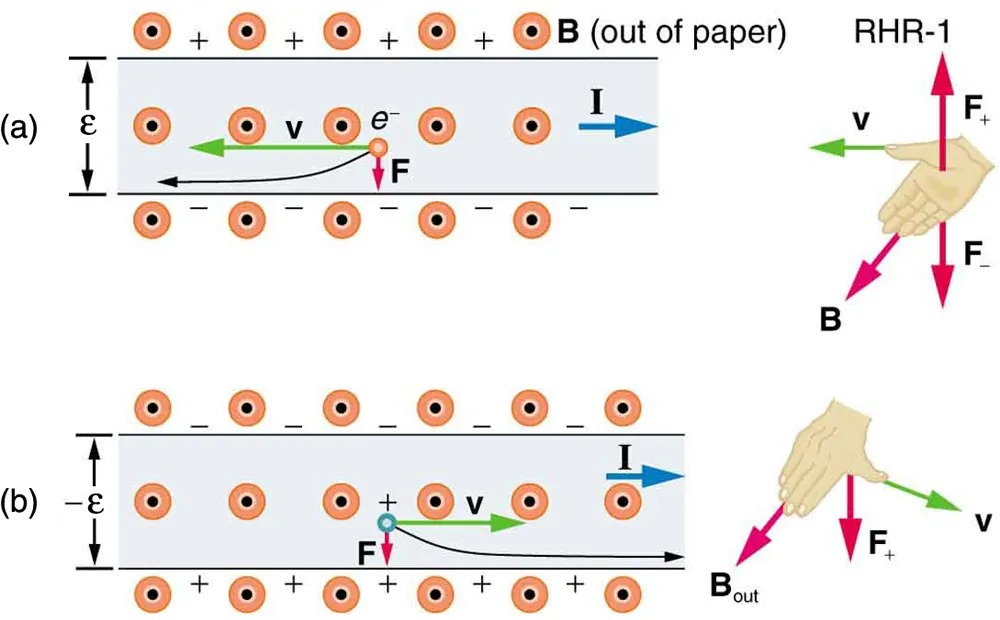
Figure 17.26 The Hall effect. (a) Electrons move to the left in this flat conductor (conventional current to the right). The magnetic field is directly out of the page, represented by circled dots; it exerts a force on the moving charges, causing a voltage [latex]\epsilon[/latex], the Hall emf, across the conductor. (b) Positive charges moving to the right (conventional current also to the right) are moved to the side, producing a Hall emf of the opposite sign, [latex]–ε[/latex]. Thus, if the direction of the field and current are known, the sign of the charge carriers can be determined from the Hall effect. Image from OpenStax College Physics 2e, CC-BY 4.0
Image Description
The image consists of two diagrams labeled as (a) and (b), illustrating the motion of charged particles in a magnetic field, with accompanying hand illustrations showing the right-hand rule (RHR-1) for determining direction of forces.
Diagram (a):
- There is a horizontal channel with upper and lower lines of positive and negative charges represented by “+” and “-” signs, respectively.
- An electron, labeled as “e–“, is moving to the left, indicated by a green arrow labeled “v”.
- A red arrow labeled “F” points downward, showing the force on the electron.
- A blue arrow labeled “I” points to the right, indicating the direction of current.
- A note indicates “B (out of paper)” representing the magnetic field direction coming out of the paper.
Diagram (b):
- Similar setup with horizontal channel and charges.
- A positive charge labeled “+” is moving to the right with a green arrow labeled “v”.
- A red arrow labeled “F” points upwards, indicating the force.
- A blue arrow labeled “I” also points to the right, indicating current direction.
- A note indicates “B (out of paper)” representing the magnetic field direction coming out of the paper.
Right-Hand Rule (RHR-1) Illustrations:
- Each diagram has an accompanying right-hand illustration to demonstrate the right-hand rule.
- For the electron, the thumb points in the direction of “v”, fingers point in the direction of “B”, and the palm faces the direction of force “F”.
- Similar setup for the positive charge with directions adjusted for opposite force direction.
One very important use of the Hall effect is to determine whether positive or negative charges carries the current. Note that in Figure 17.26(b), where positive charges carry the current, the Hall emf has the sign opposite to when negative charges carry the current. Historically, the Hall effect was used to show that electrons carry current in metals and it also shows that positive charges carry current in some semiconductors. The Hall effect is used today as a research tool to probe the movement of charges, their drift velocities and densities, and so on, in materials. In 1980, it was discovered that the Hall effect is quantized, an example of quantum behavior in a macroscopic object.
The Hall effect has other uses that range from the determination of blood flow rate to precision measurement of magnetic field strength. To examine these quantitatively, we need an expression for the Hall emf, [latex]\epsilon[/latex], across a conductor. Consider the balance of forces on a moving charge in a situation where [latex]B[/latex], [latex]v[/latex], and [latex]l[/latex] are mutually perpendicular, such as shown in Figure 17.27. Although the magnetic force moves negative charges to one side, they cannot build up without limit. The electric field caused by their separation opposes the magnetic force, [latex]F = \text{qvB}[/latex], and the electric force, [latex]F_{e} = \text{qE}[/latex], eventually grows to equal it. That is,
[latex]\text{qE} = \text{qvB}[/latex]
or
[latex]E = \text{vB} .[/latex]
Note that the electric field [latex]E[/latex] is uniform across the conductor because the magnetic field [latex]B[/latex] is uniform, as is the conductor. For a uniform electric field, the relationship between electric field and voltage is [latex]E = \epsilon / l[/latex], where [latex]l[/latex] is the width of the conductor and [latex]\epsilon[/latex] is the Hall emf. Entering this into the last expression gives
[latex]\frac{\epsilon}{l} = \text{vB} .[/latex]
Solving this for the Hall emf yields
[latex]\epsilon = \text{Blv} \left(\right. B , v , \text{and} l , \text{mutually perpendicular} \left.\right) ,[/latex]
where [latex]\epsilon[/latex] is the Hall effect voltage across a conductor of width [latex]l[/latex] through which charges move at a speed [latex]v[/latex].
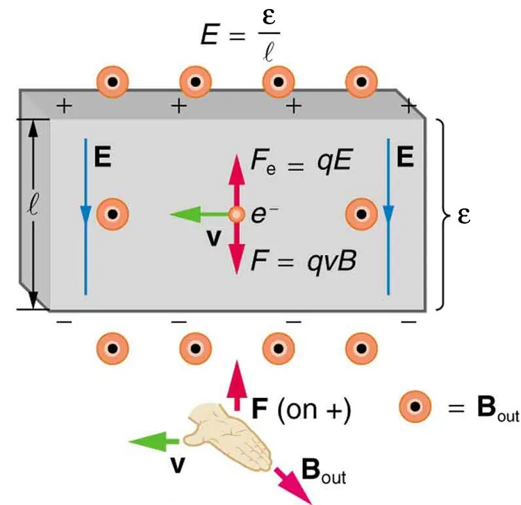
Figure 17.27 The Hall emf [latex]\epsilon[/latex] produces an electric force that balances the magnetic force on the moving charges. The magnetic force produces charge separation, which builds up until it is balanced by the electric force, an equilibrium that is quickly reached. Image from OpenStax College Physics 2e, CC-BY 4.0
Image Description
This image illustrates the concept of the Hall Effect in a conductive material. It shows a rectangular conductor placed in a magnetic field. The following elements are present in the image:
- A rectangular block labeled with dimensions l (length) and ε (electromotive force), which indicates the electric field E = ε/l.
- Positive and negative charges are depicted on the top and bottom surfaces of the block, respectively, indicating a separation of charge due to the magnetic field.
- The force on an electron e− is shown with a red arrow labeled F, with equations Fe = qE and F = qvB beside it. This depicts the electric force and magnetic force acting on a charged particle.
- The electron’s velocity v is shown with a green arrow pointing to the left.
- An illustration of a hand is used to demonstrate the right-hand rule. The thumb represents the velocity v, the fingers represent the magnetic field Bout, and the force direction F (on +) is shown with a red arrow.
This image provides a visual representation of how an external magnetic field affects the flow of electrons in a conductor, resulting in an observable Hall voltage across the conductor.
One of the most common uses of the Hall effect is in the measurement of magnetic field strength [latex]B[/latex]. Such devices, called Hall probes, can be made very small, allowing fine position mapping. Hall probes can also be made very accurate, usually accomplished by careful calibration. Another application of the Hall effect is to measure fluid flow in any fluid that has free charges (most do). (See Figure 17.28.) A magnetic field applied perpendicular to the flow direction produces a Hall emf [latex]\epsilon[/latex] as shown. Note that the sign of [latex]\epsilon[/latex] depends not on the sign of the charges, but only on the directions of [latex]B[/latex] and [latex]v[/latex]. The magnitude of the Hall emf is [latex]\epsilon = \text{Blv}[/latex], where [latex]l[/latex] is the pipe diameter, so that the average velocity [latex]v[/latex] can be determined from [latex]\epsilon[/latex] providing the other factors are known.
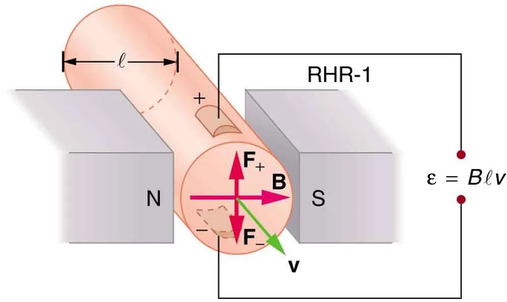
Figure 17.28 The Hall effect can be used to measure fluid flow in any fluid having free charges, such as blood. The Hall emf [latex]\epsilon[/latex] is measured across the tube perpendicular to the applied magnetic field and is proportional to the average velocity [latex]v[/latex]. Image from OpenStax College Physics 2e, CC-BY 4.0
Image Description
This image illustrates an electromagnetic induction scenario involving a metal rod positioned between the poles of a magnet. The rod is represented as a cylinder with a marked length indicated by the symbol “l.” The poles of the magnet are labeled “N” for the North pole and “S” for the South pole, positioned on opposite sides of the rod.
A schematic circuit connects the rod to a measuring device with two red connection points. The right side of the image includes the equation ɛ = Bℓv, where ɛ (epsilon) represents the electromotive force, B represents the magnetic field strength, ℓ (ell) is the length of the rod, and v is the velocity of the rod.
Arrows indicate the direction of various forces and fields:
- A pink arrow labeled “B” points horizontally across the rod, representing the magnetic field.
- A red arrow labeled “F+” points upward, indicating the force experienced by positive charges.
- A green arrow labeled “F–” points downward, indicating the force on negative charges.
- A green arrow labeled “v” points to the right, showing the direction of velocity.
A label “RHR-1” indicates the application of the right-hand rule to determine the direction of these forces. Overall, the diagram explains the concept of electromagnetic induction by showing how the motion of the rod through a magnetic field induces an electric current.
Example 17.3
Calculating the Hall emf: Hall Effect for Blood Flow
A Hall effect flow probe is placed on an artery, applying a 0.100-T magnetic field across it, in a setup similar to that in Figure 17.28. What is the Hall emf, given the vessel’s inside diameter is 4.00 mm and the average blood velocity is 20.0 cm/s?
Strategy
Because [latex]B[/latex], [latex]v[/latex], and [latex]l[/latex] are mutually perpendicular, the equation [latex]\epsilon = \text{Blv}[/latex] can be used to find [latex]\epsilon[/latex].
Solution
Entering the given values for [latex]B[/latex], [latex]v[/latex], and [latex]l[/latex] gives
[latex]\begin{eqnarray*}\epsilon & = & \text{Blv} = \left(\text{0}.\text{100 T}\right) \left(4 . \text{00} \times \text{10}^{- 3} m\right) \left(0 .\text{200 m}/\text{s}\right) \\ & = & \text{80}.\text{0 }\mu\text{V}\end{eqnarray*}[/latex]
Discussion
This is the average voltage output. Instantaneous voltage varies with pulsating blood flow. The voltage is small in this type of measurement. [latex]\epsilon[/latex] is particularly difficult to measure, because there are voltages associated with heart action (ECG voltages) that are on the order of millivolts. In practice, this difficulty is overcome by applying an AC magnetic field, so that the Hall emf is AC with the same frequency. An amplifier can be very selective in picking out only the appropriate frequency, eliminating signals and noise at other frequencies.
