17.5 Force on a Moving Charge in a Magnetic Field: Examples and Applications

Magnetic force can cause a charged particle to move in a circular or spiral path. Cosmic rays are energetic charged particles in outer space, some of which approach the Earth. They can be forced into spiral paths by the Earth’s magnetic field. Protons in giant accelerators are kept in a circular path by magnetic force. The bubble chamber photograph in Figure 17.18 shows charged particles moving in such curved paths. The curved paths of charged particles in magnetic fields are the basis of a number of phenomena and can even be used analytically, such as in a mass spectrometer.

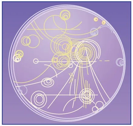
Figure 17.18 Trails of bubbles are produced by high-energy charged particles moving through the superheated liquid hydrogen in this artist’s rendition of a bubble chamber. There is a strong magnetic field perpendicular to the page that causes the curved paths of the particles. The radius of the path can be used to find the mass, charge, and energy of the particle. Image from OpenStax College Physics 2e, CC-BY 4.0

So does the magnetic force cause circular motion? Magnetic force is always perpendicular to velocity, so that it does no work on the charged particle. The particle’s kinetic energy and speed thus remain constant. The direction of motion is affected, but not the speed. This is typical of uniform circular motion. The simplest case occurs when a charged particle moves perpendicular to a uniform [latex]B[/latex]-field, such as shown in Figure 17.19. (If this takes place in a vacuum, the magnetic field is the dominant factor determining the motion.) Here, the magnetic force supplies the centripetal force [latex]F_{c} = \text{mv}^{2} / r[/latex]. Noting that [latex]\text{sin} \theta = 1[/latex], we see that [latex]F = \text{qvB}[/latex].

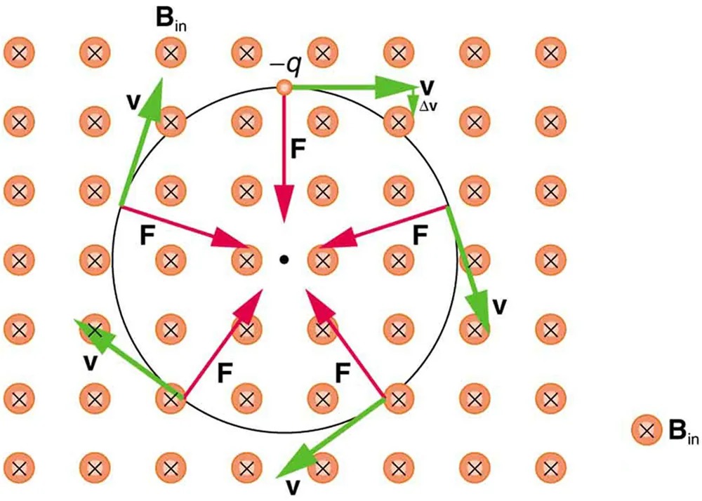
Figure 17.19 A negatively charged particle moves in the plane of the page in a region where the magnetic field is perpendicular into the page (represented by the small circles with x’s—like the tails of arrows). The magnetic force is perpendicular to the velocity, and so velocity changes in direction but not magnitude. Uniform circular motion results. Image from OpenStax College Physics 2e, CC-BY 4.0

Because the magnetic force [latex]F[/latex] supplies the centripetal force [latex]F_{c}[/latex], we have

Solving for [latex]r[/latex] yields

Here, [latex]r[/latex] is the radius of curvature of the path of a charged particle with mass [latex]m[/latex] and charge [latex]q[/latex], moving at a speed [latex]v[/latex] perpendicular to a magnetic field of strength [latex]B[/latex]. If the velocity is not perpendicular to the magnetic field, then [latex]v[/latex] is the component of the velocity perpendicular to the field. The component of the velocity parallel to the field is unaffected, since the magnetic force is zero for motion parallel to the field. This produces a spiral motion rather than a circular one.

Example 17.2

Calculating the Curvature of the Path of an Electron Moving in a Magnetic Field: A Magnet on a TV Screen

A magnet brought near an old-fashioned TV screen such as in Figure 17.20 (TV sets with cathode ray tubes instead of LCD screens) severely distorts its picture by altering the path of the electrons that make its phosphors glow. (Don’t try this at home, as it will permanently magnetize and ruin the TV.) To illustrate this, calculate the radius of curvature of the path of an electron having a velocity of [latex]6 . \text{00} \times \text{10}^{7} \text{m}/\text{s}[/latex] (corresponding to the accelerating voltage of about 10.0 kV used in some TVs) perpendicular to a magnetic field of strength [latex]B = 0 .\text{500 T}[/latex] (obtainable with permanent magnets).

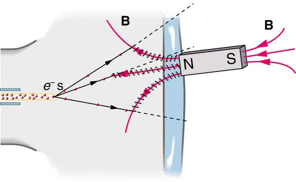
Figure 17.20 Side view showing what happens when a magnet comes in contact with a computer monitor or TV screen. Electrons moving toward the screen spiral about magnetic field lines, maintaining the component of their velocity parallel to the field lines. This distorts the image on the screen. Image from OpenStax College Physics 2e, CC-BY 4.0

Image Description

The image is a diagram illustrating the behavior of electrons within a magnetic field. On the left side, a stream of electrons, indicated by the symbol “e^–“, is shown moving from left to right. The electrons are depicted as small, red spheres within a pale yellow beam.

The beam of electrons enters a region with a magnetic field represented by the letter “B”. The magnetic field lines are shown as curved red arrows entering and exiting a rectangular magnet. The magnet is oriented with its north (N) and south (S) poles facing sideways, relative to the electron beam.

As the electrons enter the magnetic field, they follow curved, parabolic trajectories. Three distinct paths are illustrated with dashed black lines and arrows, depicting how the electron paths are bent differently as they pass through the magnetic field.

Strategy

We can find the radius of curvature [latex]r[/latex] directly from the equation [latex]r = \frac{m v}{q B}[/latex], since all other quantities in it are given or known.

Solution

Using known values for the mass and charge of an electron, along with the given values of [latex]v[/latex] and [latex]B[/latex] gives us

[latex]\begin{eqnarray*}r = \frac{\text{mv}}{\text{qB}} & = & \frac{\left(9 . \text{11} \times \text{10}^{- \text{31}} \text{kg}\right) \left(6 . \text{00} \times \text{10}^{7} \text{m}/\text{s}\right)}{\left(1 . \text{60} \times \text{10}^{- \text{19}} \text{C}\right) \left(0 . \text{500} \text{T}\right)} \\ & = & 6 . \text{83} \times \text{10}^{- 4} \text{m}\end{eqnarray*}[/latex]

17.8

or

[latex]r = 0 . \text{683 mm} .[/latex]

17.9

Discussion

The small radius indicates a large effect. The electrons in the TV picture tube are made to move in very tight circles, greatly altering their paths and distorting the image.

Figure 17.21 shows how electrons not moving perpendicular to magnetic field lines follow the field lines. The component of velocity parallel to the lines is unaffected, and so the charges spiral along the field lines. If field strength increases in the direction of motion, the field will exert a force to slow the charges, forming a kind of magnetic mirror, as shown below.

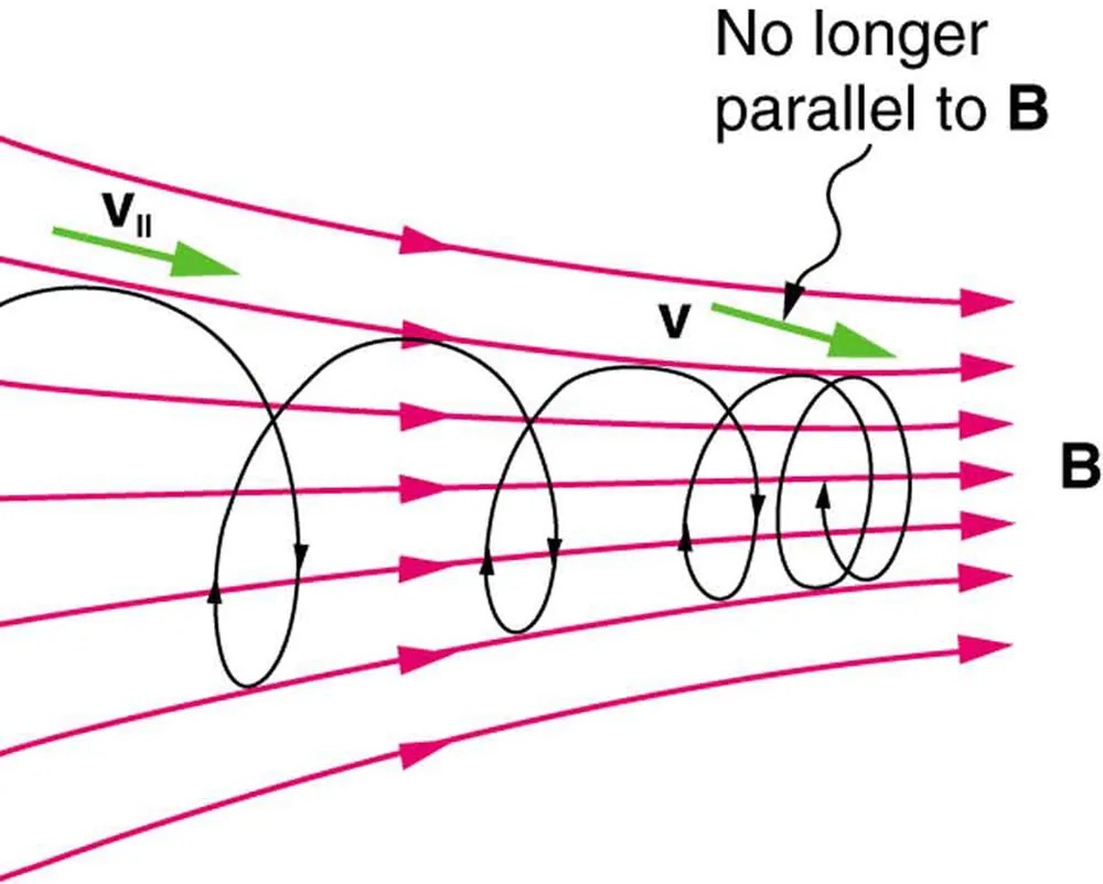
Figure 17.21 When a charged particle moves along a magnetic field line into a region where the field becomes stronger, the particle experiences a force that reduces the component of velocity parallel to the field. This force slows the motion along the field line and here reverses it, forming a “magnetic mirror.” Image from OpenStax College Physics 2e, CC-BY 4.0

The properties of charged particles in magnetic fields are related to such different things as the Aurora Australis or Aurora Borealis and particle accelerators. Charged particles approaching magnetic field lines may get trapped in spiral orbits about the lines rather than crossing them, as seen above. Some cosmic rays, for example, follow the Earth’s magnetic field lines, entering the atmosphere near the magnetic poles and causing the southern or northern lights through their ionization of molecules in the atmosphere. This glow of energized atoms and molecules is seen in Introduction to Magnetism. Those particles that approach middle latitudes must cross magnetic field lines, and many are prevented from penetrating the atmosphere. Cosmic rays are a component of background radiation; consequently, they give a higher radiation dose at the poles than at the equator.

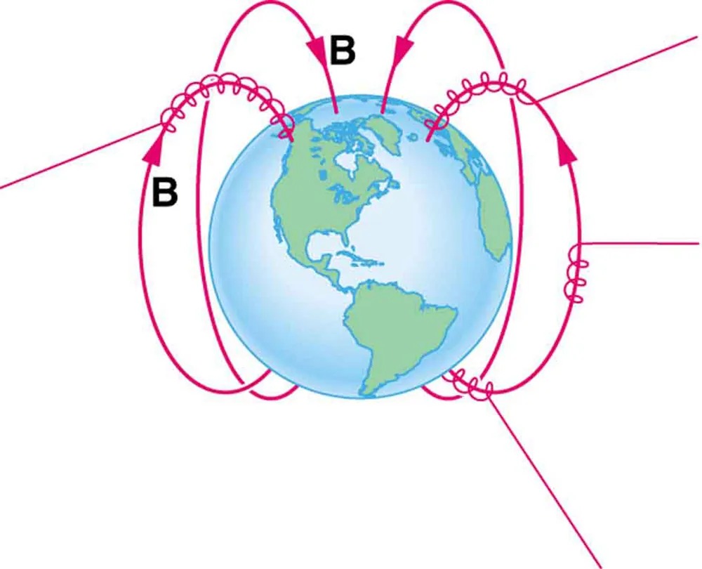
Figure 17.22 Energetic electrons and protons, components of cosmic rays, from the Sun and deep outer space often follow the Earth’s magnetic field lines rather than cross them. Image from OpenStax College Physics 2e, CC-BY 4.0

Some incoming charged particles become trapped in the Earth’s magnetic field, forming two belts above the atmosphere known as the Van Allen radiation belts after the discoverer James A. Van Allen, an American astrophysicist. (See Figure 17.23.) Particles trapped in these belts form radiation fields (similar to nuclear radiation) so intense that piloted space flights avoid them and satellites with sensitive electronics are kept out of them. In the few minutes it took lunar missions to cross the Van Allen radiation belts, astronauts received radiation doses more than twice the allowed annual exposure for radiation workers. Other planets have similar belts, especially those having strong magnetic fields like Jupiter.

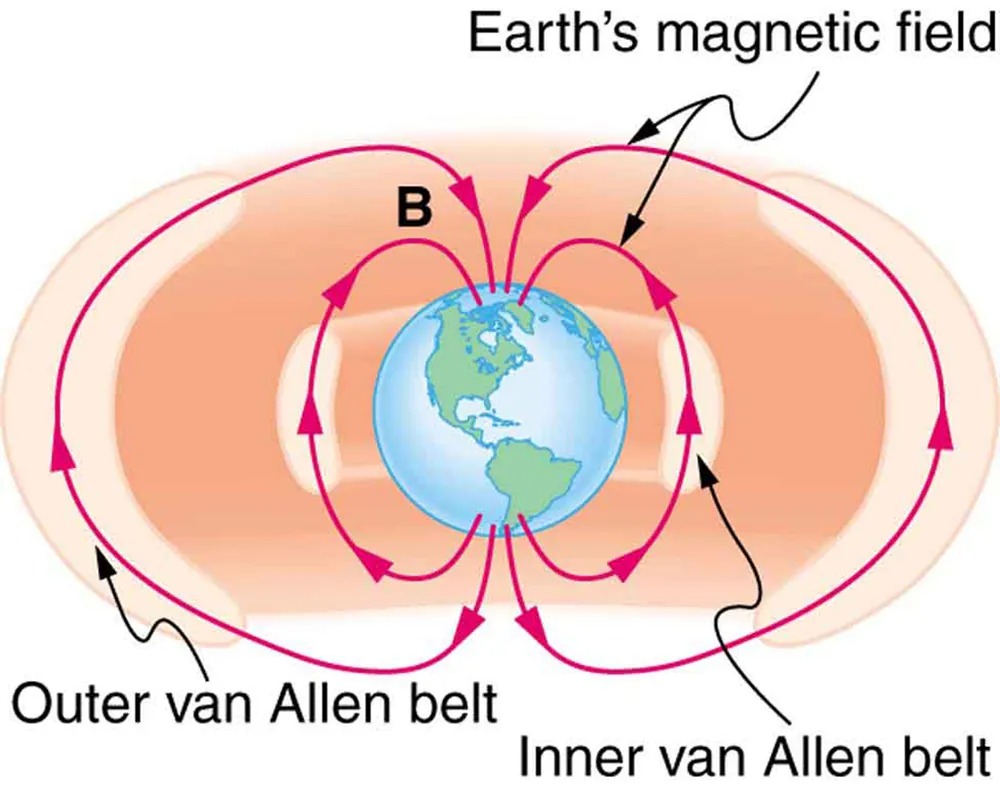
Figure 17.23 The Van Allen radiation belts are two regions in which energetic charged particles are trapped in the Earth’s magnetic field. One belt lies about 300 km above the Earth’s surface, the other about 16,000 km. Charged particles in these belts migrate along magnetic field lines and are partially reflected away from the poles by the stronger fields there. The charged particles that enter the atmosphere are replenished by the Sun and sources in deep outer space. Image from OpenStax College Physics 2e, CC-BY 4.0

Back on Earth, we have devices that employ magnetic fields to contain charged particles. Among them are the giant particle accelerators that have been used to explore the substructure of matter. (See Figure 17.24.) Magnetic fields not only control the direction of the charged particles, they also are used to focus particles into beams and overcome the repulsion of like charges in these beams.

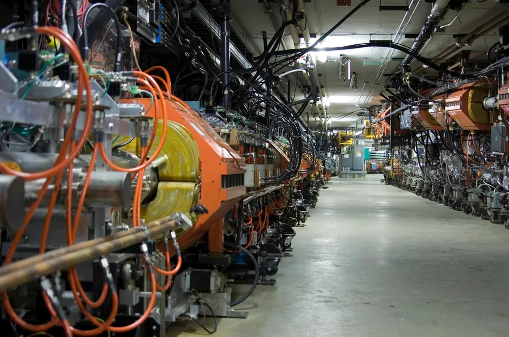
Figure 17.24 The Fermilab facility in Illinois has a large particle accelerator (the most powerful in the world until 2008) that employs magnetic fields (magnets seen here in orange) to contain and direct its beam. This and other accelerators have been in use for several decades and have allowed us to discover some of the laws underlying all matter. Image from OpenStax College Physics 2e, CC-BY 4.0

Thermonuclear fusion (like that occurring in the Sun) is a hope for a future clean energy source. One of the most promising devices is the tokamak, which uses magnetic fields to contain (or trap) and direct the reactive charged particles. (See Figure 17.25.) Less exotic, but more immediately practical, amplifiers in microwave ovens use a magnetic field to contain oscillating electrons. These oscillating electrons generate the microwaves sent into the oven.

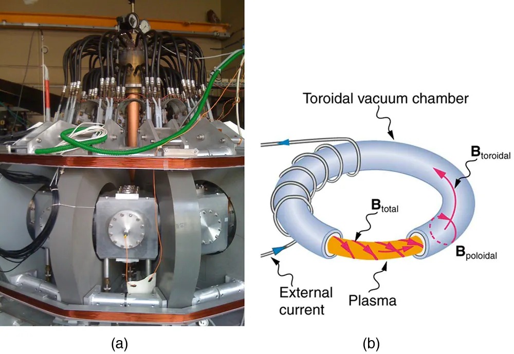
Figure 17.25 Tokamaks such as the one shown in the figure are being studied with the goal of economical production of energy by nuclear fusion. Magnetic fields in the doughnut-shaped device contain and direct the reactive charged particles. Image from OpenStax College Physics 2e, CC-BY 4.0

Mass spectrometers have a variety of designs, and many use magnetic fields to measure mass. The curvature of a charged particle’s path in the field is related to its mass and is measured to obtain mass information. (See More Applications of Magnetism.) Historically, such techniques were employed in the first direct observations of electron charge and mass. Today, mass spectrometers (sometimes coupled with gas chromatographs) are used to determine the make-up and sequencing of large biological molecules.