16.5 Alternating Current versus Direct Current
Learning Objectives
By the end of this section, you will be able to:
- Explain the differences and similarities between AC and DC current.
- Calculate rms voltage, current, and average power.
- Explain why AC current is used for power transmission.
Alternating Current
Most of the examples dealt with so far, and particularly those utilizing batteries, have constant voltage sources. Once the current is established, it is thus also a constant. Direct current (DC) is the flow of electric charge in only one direction. It is the steady state of a constant-voltage circuit. Most well-known applications, however, use a time-varying voltage source. Alternating current (AC) is the flow of electric charge that periodically reverses direction. If the source varies periodically, particularly sinusoidally, the circuit is known as an alternating current circuit. Examples include the commercial and residential power that serves so many of our needs. Figure 16.14 shows graphs of voltage and current versus time for typical DC and AC power. The AC voltages and frequencies commonly used in homes and businesses vary around the world.
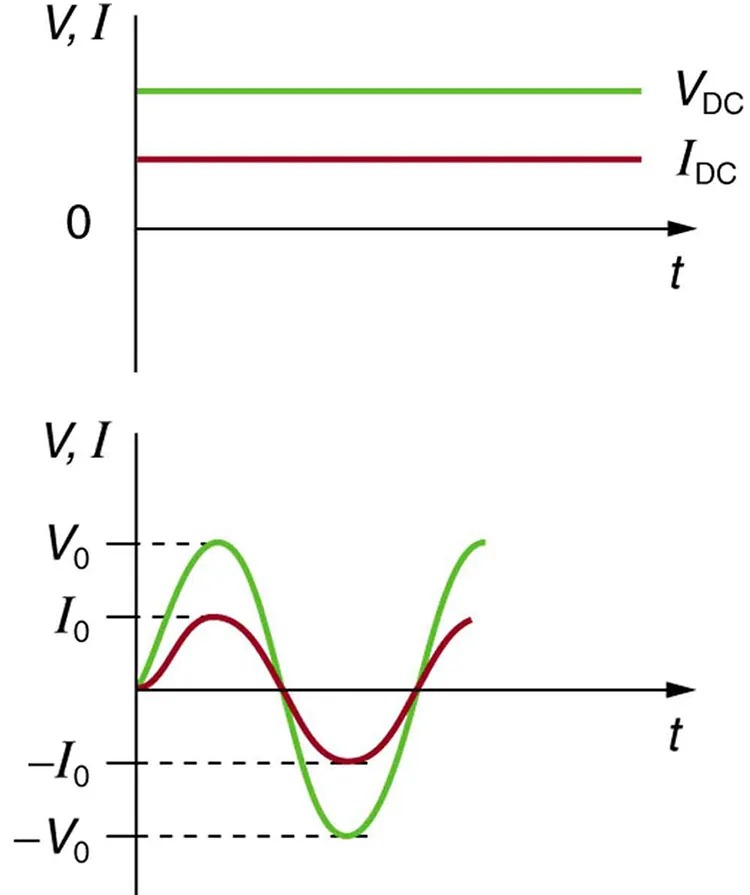
Figure 16.14 (a) DC voltage and current are constant in time, once the current is established. (b) A graph of voltage and current versus time for 60-Hz AC power. The voltage and current are sinusoidal and are in phase for a simple resistance circuit. The frequencies and peak voltages of AC sources differ greatly. Image from OpenStax College Physics 2e, CC-BY 4.0
Image Description
The image consists of two graphs depicting voltage and current over time.
The top graph shows a Direct Current (DC) representation. It has a horizontal axis labeled “t” for time, and a vertical axis labeled “V, I” for voltage and current. Two straight horizontal lines are in the graph: a green line labeled “VDC” and a red line labeled “IDC“, both lines are parallel to the time axis, indicating constant voltage and current.
The bottom graph shows an Alternating Current (AC) representation. It also has a horizontal axis labeled “t” and a vertical axis labeled “V, I”. The graph contains two sinusoidal waves: a green wave representing voltage and a red wave representing current. These waves oscillate above and below the horizontal axis. Key points along the vertical axis are marked with dashed lines and labeled as “V0“, “I0“, “-I0“, and “-V0“, indicating the peak and negative peak values of the waveform.
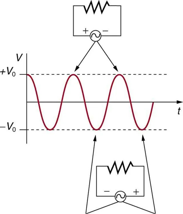
Figure 16.15 The potential difference [latex]V[/latex] between the terminals of an AC voltage source fluctuates as shown. The mathematical expression for [latex]V[/latex] is given by [latex]V = V_{0} \text{sin} \text{ 2 } \pi \text{ft}[/latex]. Image from OpenStax College Physics 2e, CC-BY 4.0
Image Description
The image illustrates an electrical circuit and waveform diagram. At the top, there is a diagram of an electrical circuit containing a resistor connected in series with an AC voltage source indicated by a sine wave symbol with positive and negative terminals.
Below the circuit diagram is a graph showing a sinusoidal waveform. The graph has a vertical axis labeled ‘V’ and a horizontal axis labeled ‘t’. The waveform oscillates symmetrically around the horizontal center line.
The maximum and minimum values of the waveform are marked by dashed lines labeled ‘+V0‘ and ‘-V0‘, respectively. Arrows point from the circuit diagram to the positive and negative peaks of the waveform.
A similar circuit diagram is repeated at the bottom, inverted in orientation, with arrows pointing upwards towards the graph.
Figure 16.15 shows a schematic of a simple circuit with an AC voltage source. The voltage between the terminals fluctuates as shown, with the AC voltage given by
[latex]V = V_{0} \text{sin} \text{ 2} \pi \text{ft},[/latex]
where [latex]V[/latex] is the voltage at time [latex]t[/latex], [latex]V_{0}[/latex] is the peak voltage, and [latex]f[/latex] is the frequency in hertz. For this simple resistance circuit, [latex]I = \text{V}/\text{R}[/latex], and so the AC current is
[latex]I = I_{0} \text{ sin 2} \pi \text{ft},[/latex]
where [latex]I[/latex] is the current at time [latex]t[/latex], and [latex]I_{0} = V_{0} /\text{R}[/latex] is the peak current. For this example, the voltage and current are said to be in phase, as seen in Figure 16.14(b).
Current in the resistor alternates back and forth just like the driving voltage, since [latex]I = \text{V}/\text{R}[/latex]. If the resistor is a fluorescent light bulb, for example, it brightens and dims 120 times per second as the current repeatedly goes through zero. A 120-Hz flicker is too rapid for your eyes to detect, but if you wave your hand back and forth between your face and a fluorescent light, you will see a stroboscopic effect evidencing AC. The fact that the light output fluctuates means that the power is fluctuating. The power supplied is [latex]P = \text{IV}[/latex]. Using the expressions for [latex]I[/latex] and [latex]V[/latex] above, we see that the time dependence of power is [latex]P = I_{0} V_{0} \text{sin}^{2} \text{ 2} \pi \text{ft}[/latex], as shown in Figure 16.16.
Making Connections: Take-Home Experiment—AC/DC Lights
Wave your hand back and forth between your face and a fluorescent light bulb. Do you observe the same thing with the headlights on your car? Explain what you observe. Warning: Do not look directly at very bright light.
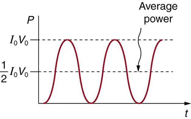
Figure 16.16 AC power as a function of time. Since the voltage and current are in phase here, their product is non-negative and fluctuates between zero and [latex]I_{0} V_{0}[/latex]. Average power is [latex]\left(\right. 1 / 2 \left.\right) I_{0} V_{0}[/latex]. Image from OpenStax College Physics 2e, CC-BY 4.0
Image Description
The image is a graph showing a waveform representing power over time. The horizontal axis is labeled “t” for time, and the vertical axis is labeled “P” for power. The waveform is sinusoidal, oscillating between two levels: a higher level labeled as “I0V0” and a lower level labeled as “1/2 I0V0“. A dashed horizontal line indicates the average power level, which is also marked on the graph. An arrow points to this average level with the text “Average power.”
We are most often concerned with average power rather than its fluctuations—that 60-W light bulb in your desk lamp has an average power consumption of 60 W, for example. As illustrated in Figure 16.16, the average power [latex]P_{\text{ave}}[/latex] is
[latex]P_{\text{ave}} = \frac{1}{2} I_{0} V_{0} .[/latex]
This is evident from the graph, since the areas above and below the [latex]\left(\right. 1 / 2 \left.\right) I_{0} V_{0}[/latex] line are equal, but it can also be proven using trigonometric identities. Similarly, we define an average or rms current [latex]I_{\text{rms}}[/latex] and average or rms voltage [latex]V_{\text{rms}}[/latex] to be, respectively,
[latex]I_{\text{rms }} = \frac{I_{0}}{\sqrt{2}}[/latex]
and
[latex]V_{\text{rms }} = \frac{V_{0}}{\sqrt{2}} .[/latex]
where rms stands for root mean square, a particular kind of average. In general, to obtain a root mean square, the particular quantity is squared, its mean (or average) is found, and the square root is taken. This is useful for AC, since the average value is zero. Now,
[latex]P_{\text{ave}} = I_{\text{rms}} V_{\text{rms}} ,[/latex]
which gives
[latex]P_{\text{ave}} = \frac{I_{0}}{\sqrt{2}} \cdot \frac{V_{0}}{\sqrt{2}} = \frac{1}{2} I_{0} V_{0} ,[/latex]
as stated above. It is standard practice to quote [latex]I_{\text{rms}}[/latex], [latex]V_{\text{rms}}[/latex], and [latex]P_{\text{ave}}[/latex] rather than the peak values. For example, most household electricity is 120 V AC, which means that [latex]V_{\text{rms}}[/latex] is 120 V. The common 10-A circuit breaker will interrupt a sustained [latex]I_{\text{rms}}[/latex] greater than 10 A. Your 1.0-kW microwave oven consumes [latex]P_{\text{ave}} = \text{1}.\text{0 kW}[/latex], and so on. You can think of these rms and average values as the equivalent DC values for a simple resistive circuit.
To summarize, when dealing with AC, Ohm’s law and the equations for power are completely analogous to those for DC, but rms and average values are used for AC. Thus, for AC, Ohm’s law is written
[latex]I_{\text{rms}} = \frac{V_{\text{rms}}}{R} .[/latex]
The various expressions for AC power [latex]P_{\text{ave}}[/latex] are
[latex]P_{\text{ave}} = I_{\text{rms}} V_{\text{rms}} ,[/latex]
[latex]P_{\text{ave}} = \frac{V_{\text{rms}}^{2}}{R} ,[/latex]
and
[latex]P_{\text{ave}} = I_{\text{rms}}^{2} R .[/latex]
Example 16.9
Peak Voltage and Power for AC
(a) What is the value of the peak voltage for 120-V AC power? (b) What is the peak power consumption rate of a 60.0-W AC light bulb?
Strategy
We are told that [latex]V_{\text{rms}}[/latex] is 120 V and [latex]P_{\text{ave}}[/latex] is 60.0 W. We can use [latex]V_{\text{rms }} = \frac{V_{0}}{\sqrt{2}}[/latex] to find the peak voltage, and we can manipulate the definition of power to find the peak power from the given average power.
Solution for (a)
Solving the equation [latex]V_{\text{rms }} = \frac{V_{0}}{\sqrt{2}}[/latex] for the peak voltage [latex]V_{0}[/latex] and substituting the known value for [latex]V_{\text{rms}}[/latex] gives
[latex]V_{0} = \sqrt{2} V_{\text{rms}} = \text{ 1} . \text{414} \left(\right. \text{120 V} \left.\right) = \text{ 170 V} .[/latex]
Discussion for (a)
This means that the AC voltage swings from 170 V to [latex]–\text{170 V}[/latex] and back 60 times every second. An equivalent DC voltage is a constant 120 V.
Solution for (b)
Peak power is peak current times peak voltage. Thus,
[latex]P_{0} = I_{0} V_{0} = \text{ 2} \left(\frac{1}{2} I_{0} V_{0}\right) = \text{ 2} P_{\text{ave}} .[/latex]
We know the average power is 60.0 W, and so
[latex]P_{0} = \text{ 2} \left(\right. \text{60} . \text{0 W} \left.\right) = \text{ 120 W} .[/latex]
Discussion
So the power swings from zero to 120 W one hundred twenty times per second (twice each cycle), and the power averages 60 W.
Why Use AC for Power Distribution?
Most large power-distribution systems are AC. Moreover, the power is transmitted at much higher voltages than the 120-V AC (240 V in most parts of the world) we use in homes and on the job. Economies of scale make it cheaper to build a few very large electric power-generation plants than to build numerous small ones. This necessitates sending power long distances, and it is obviously important that energy losses en route be minimized. High voltages can be transmitted with much smaller power losses than low voltages, as we shall see. (See Figure 16.17.) For safety reasons, the voltage at the user is reduced to familiar values. The crucial factor is that it is much easier to increase and decrease AC voltages than DC, so AC is used in most large power distribution systems.
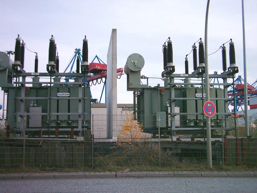
Figure 16.17 Power is distributed over large distances at high voltage to reduce power loss in the transmission lines. The voltages generated at the power plant are stepped up by passive devices called transformers (see ) to 330,000 volts (or more in some places worldwide). At the point of use, the transformers reduce the voltage transmitted for safe residential and commercial use. Image from OpenStax College Physics 2e, CC-BY 4.0
Example 16.10
Power Losses Are Less for High-Voltage Transmission
(a) What current is needed to transmit 100 MW of power at 200 kV? (b) What is the power dissipated by the transmission lines if they have a resistance of [latex]1 . \text{00} \Omega[/latex]? (c) What percentage of the power is lost in the transmission lines?
Strategy
We are given [latex]P_{\text{ave}} = \text{100 MW}[/latex], [latex]V_{\text{rms}} = \text{200 kV}[/latex], and the resistance of the lines is [latex]R = 1 . \text{00} \Omega[/latex]. Using these givens, we can find the current flowing (from [latex]P = \text{IV}[/latex]) and then the power dissipated in the lines ([latex]P = I^{2} R[/latex]), and we take the ratio to the total power transmitted.
Solution
To find the current, we rearrange the relationship [latex]P_{\text{ave}} = I_{\text{rms}} V_{\text{rms}}[/latex] and substitute known values. This gives
[latex]I_{\text{rms}} = \frac{P_{\text{ave}}}{V_{\text{rms}}} = \frac{\text{100 } \times \text{ 10}^{6} \text{ W}}{\text{200 } \times \text{ 10}^{3} \text{ V}} = \text{ 500 A} .[/latex]
Solution
Knowing the current and given the resistance of the lines, the power dissipated in them is found from [latex]P_{\text{ave}} = I_{\text{rms}}^{2} R[/latex]. Substituting the known values gives
[latex]P_{\text{ave}} = I_{\text{rms}}^{2} R = \left(\right. \text{500 A} \left.\right)^{2} \left(\right. 1 . \text{00 } \Omega \left.\right) = \text{ 250 kW} .[/latex]
Solution
The percent loss is the ratio of this lost power to the total or input power, multiplied by 100:
[latex]\%\text{ loss}= \frac{\text{250 kW}}{\text{100 MW}} \times \text{100} = 0 . \text{250 }\% .[/latex]
Discussion
One-fourth of a percent is an acceptable loss. Note that if 100 MW of power had been transmitted at 25 kV, then a current of 4000 A would have been needed. This would result in a power loss in the lines of 16.0 MW, or 16.0% rather than 0.250%. The lower the voltage, the more current is needed, and the greater the power loss in the fixed-resistance transmission lines. Of course, lower-resistance lines can be built, but this requires larger and more expensive wires. If superconducting lines could be economically produced, there would be no loss in the transmission lines at all. But, as we shall see in a later chapter, there is a limit to current in superconductors, too. In short, high voltages are more economical for transmitting power, and AC voltage is much easier to raise and lower, so that AC is used in most large-scale power distribution systems.
It is widely recognized that high voltages pose greater hazards than low voltages. But, in fact, some high voltages, such as those associated with common static electricity, can be harmless. So it is not voltage alone that determines a hazard. It is not so widely recognized that AC shocks are often more harmful than similar DC shocks. Thomas Edison thought that AC shocks were more harmful and set up a DC power-distribution system in New York City in the late 1800s. There were bitter fights, in particular between Edison and George Westinghouse and Nikola Tesla, who were advocating the use of AC in early power-distribution systems. AC has prevailed largely due to transformers and lower power losses with high-voltage transmission.
PhET Explorations
Generator
Generate electricity with a bar magnet! Discover the physics behind the phenomena by exploring magnets and how you can use them to make a bulb light.
