13.7 Damped Harmonic Motion
Learning Objectives
By the end of this section, you will be able to:
- Compare and discuss underdamped and overdamped oscillating systems.
- Explain critically damped system.

Figure 13.19 In order to counteract dampening forces, this mom needs to keep pushing the swing. Image from OpenStax College Physics 2e, CC-BY 4.0
A guitar string stops oscillating a few seconds after being plucked. To keep a child happy on a swing, you must keep pushing. Although we can often make friction and other non-conservative forces negligibly small, completely undamped motion is rare. In fact, we may even want to damp oscillations, such as with car shock absorbers.
For a system that has a small amount of damping, the period and frequency are nearly the same as for simple harmonic motion, but the amplitude gradually decreases as shown in Figure 13.20. This occurs because the non-conservative damping force removes energy from the system, usually in the form of thermal energy. In general, energy removal by non-conservative forces is described as
[latex]W_{\text{nc}} = Δ \left(\right. \text{KE} + \text{PE} \left.\right) ,[/latex]
where [latex]W_{\text{nc}}[/latex] is work done by a non-conservative force (here the damping force). For a damped harmonic oscillator, [latex]W_{\text{nc}}[/latex] is negative because it removes mechanical energy (KE + PE) from the system.
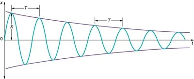
Figure 13.20 In this graph of displacement versus time for a harmonic oscillator with a small amount of damping, the amplitude slowly decreases, but the period and frequency are nearly the same as if the system were completely undamped. Image from OpenStax College Physics 2e, CC-BY 4.0
Image Description
The image depicts a graph that represents a damped wave. The horizontal axis is labeled ‘t’, possibly indicating time, while the vertical axis is labeled ‘x’. The wave begins with a larger amplitude on the left, which gradually decreases as it moves to the right. Over the wave, two points are marked, with a horizontal distance between them labeled ‘T’, which could indicate the period of the wave. The wave oscillates between two lines that converge toward the right side of the graph, indicating the damping effect. The amplitude ‘X’ at the start of the wave near the vertical axis is highlighted.
If you gradually increase the amount of damping in a system, the period and frequency begin to be affected, because damping opposes and hence slows the back and forth motion. (The net force is smaller in both directions.) If there is very large damping, the system does not even oscillate—it slowly moves toward equilibrium. Figure 13.21 shows the displacement of a harmonic oscillator for different amounts of damping. When we want to damp out oscillations, such as in the suspension of a car, we may want the system to return to equilibrium as quickly as possible Critical damping is defined as the condition in which the damping of an oscillator results in it returning as quickly as possible to its equilibrium position. The critically damped system may overshoot the equilibrium position, but if it does, it will do so only once. Critical damping is represented by Curve A in Figure 13.21. With less-than critical damping, the system will return to equilibrium faster but will overshoot and cross over one or more times. Such a system is underdamped; its displacement is represented by the curve in Figure 13.20. Curve B in Figure 13.21 represents an overdamped system. As with critical damping, it too may overshoot the equilibrium position, but will reach equilibrium over a longer period of time.
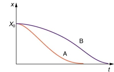
Figure 13.21 Displacement versus time for a critically damped harmonic oscillator (A) and an overdamped harmonic oscillator (B). The critically damped oscillator returns to equilibrium at [latex]X = 0[/latex] in the smallest time possible without overshooting. Image from OpenStax College Physics 2e, CC-BY 4.0
Image Description
The image is a graph with labeled axes and two curves. The horizontal axis is labeled “t” and represents time, while the vertical axis is labeled “x” and represents a variable. The point where the axes intersect is labeled “X₀”. There are two curves on the graph:
- The first curve is orange and labeled “A”. It starts at point “X₀” on the vertical axis and decreases sharply as it moves to the right along the horizontal axis.
- The second curve is purple and labeled “B”. It also starts at point “X₀” on the vertical axis but decreases more gradually compared to curve “A” as it moves to the right along the horizontal axis.
The two curves demonstrate different rates of decline over time, with curve “A” having a steeper descent than curve “B”.
Critical damping is often desired, because such a system returns to equilibrium rapidly and remains at equilibrium as well. In addition, a constant force applied to a critically damped system moves the system to a new equilibrium position in the shortest time possible without overshooting or oscillating about the new position. For example, when you stand on bathroom scales that have a needle gauge, the needle moves to its equilibrium position without oscillating. It would be quite inconvenient if the needle oscillated about the new equilibrium position for a long time before settling. Damping forces can vary greatly in character. Friction, for example, is sometimes independent of velocity (as assumed in most places in this text). But many damping forces depend on velocity—sometimes in complex ways, sometimes simply being proportional to velocity.
Example 13.7
Damping an Oscillatory Motion: Friction on an Object Connected to a Spring
Damping oscillatory motion is important in many systems, and the ability to control the damping is even more so. This is generally attained using non-conservative forces such as the friction between surfaces, and viscosity for objects moving through fluids. The following example considers friction. Suppose a 0.200-kg object is connected to a spring as shown in Figure 13.22, but there is simple friction between the object and the surface, and the coefficient of friction [latex]\mu_{k}[/latex] is equal to 0.0800. (a) What is the frictional force between the surfaces? (b) What total distance does the object travel if it is released 0.100 m from equilibrium, starting at [latex]v = 0[/latex]? The force constant of the spring is [latex]k = \text{50} . 0 N/m[/latex].
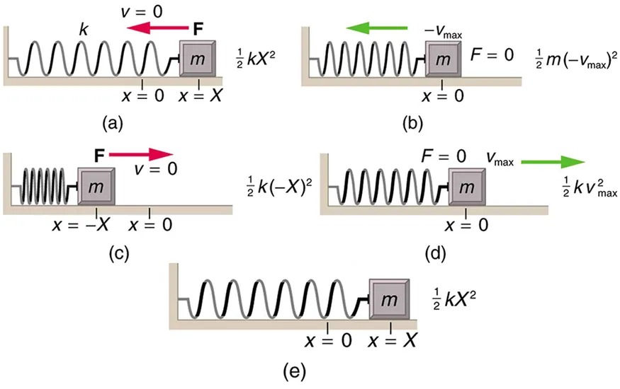
Figure 13.22 The transformation of energy in simple harmonic motion is illustrated for an object attached to a spring on a frictionless surface. Image from OpenStax College Physics 2e, CC-BY 4.0
Image Description
The image depicts five diagrams labeled (a) to (e), showing a mass-spring system in different stages of oscillation. Each diagram includes a spring constant (k), a mass (m), positions (x = 0, x = X, and x = -X), velocity (v), and force (F). Here is a description of each diagram:
(a) The mass is at position x = X with velocity v = 0. An external force F is applied to the right. The potential energy is 1/2 kX².
(b) The mass is at position x = 0. Velocity is -vmax to the left, and F = 0. The kinetic energy is 1/2 m(-vmax)².
(c) The mass is at position x = -X with velocity v = 0. An external force F is applied to the right. The potential energy is 1/2 k(-X)².
(d) The mass returns to position x = 0. Velocity is vmax to the right, and F = 0. The kinetic energy is 1/2 k vmax².
(e) The mass is back at position x = X. Energy is stored as potential energy 1/2 kX². The diagram shows equilibrium without motion.
Strategy
This problem requires you to integrate your knowledge of various concepts regarding waves, oscillations, and damping. To solve an integrated concept problem, you must first identify the physical principles involved. Part (a) is about the frictional force. This is a topic involving the application of Newton’s Laws. Part (b) requires an understanding of work and conservation of energy, as well as some understanding of horizontal oscillatory systems.
Now that we have identified the principles we must apply in order to solve the problems, we need to identify the knowns and unknowns for each part of the question, as well as the quantity that is constant in Part (a) and Part (b) of the question.
Solution a
- Choose the proper equation: Friction is [latex]f = \mu_{k} \text{mg}[/latex].
- Identify the known values.
- Enter the known values into the equation:
[latex]f = (\text{0}.\text{0800}) (0 .\text{200 kg}) (9 .\text{80 m} / \text{s}^{\text{2}} ) .[/latex]
13.58 - Calculate and convert units:
[latex]f = \text{0}.\text{157 N} .[/latex]
Discussion a
The force here is small because the system and the coefficients are small.
Solution b
Identify the known:
- The system involves elastic potential energy as the spring compresses and expands, friction that is related to the work done, and the kinetic energy as the body speeds up and slows down.
- Energy is not conserved as the mass oscillates because friction is a non-conservative force.
- The motion is horizontal, so gravitational potential energy does not need to be considered.
- Because the motion starts from rest, the energy in the system is initially [latex]\text{PE}_{el,i} = \left(\right. 1 / 2 \left.\right) \text{kX}^{2}[/latex]. This energy is removed by work done by friction [latex]W_{\text{nc}} = – \text{fd}[/latex], where [latex]d[/latex] is the total distance traveled and [latex]f = \mu_{\text{k}} \text{mg}[/latex] is the force of friction. When the system stops moving, the friction force will balance the force exerted by the spring, so [latex]\text{PE }_{\text{e1},\text{f }} = \left(\right. 1 / 2 \left.\right) \text{kx }^{2}[/latex] where [latex]x[/latex] is the final position and is given by
[latex]\begin{eqnarray*}F_{\text{el}} & = & f \\ \text{kx} & = & \mu_{\text{k}} \text{mg} \\ x & = & \frac{\mu_{\text{k}} \text{mg}}{k} .\end{eqnarray*}[/latex]
13.59
- By equating the work done to the energy removed, solve for the distance
[latex]d[/latex]
. - The work done by the non-conservative forces equals the initial, stored elastic potential energy. Identify the correct equation to use:
[latex]\begin{align*}\text{W }_{\text{nc }} &= \Delta \left(\text{KE } + \text{PE }\right)\\ &= \text{PE }_{\text{el},\text{f }} - \text{PE }_{\text{el},\text{i }} \\&= \frac{1}{2} k \left(\left(\frac{\mu_{k} \textit{mg }}{k}\right)^{2} - X^{2}\right) .\end{align*}[/latex]
13.60 - Recall that [latex]W_{\text{nc}} = – \text{fd}[/latex].
- Enter the friction as [latex]f = \mu_{\text{k}} \text{mg}[/latex] into [latex]W_{\text{nc}} = – \text{fd}[/latex], thus
[latex]W_{\text{nc}} = \left(– \mu\right)_{\text{k}} \text{mgd} .[/latex]
13.61 - Combine these two equations to find
[latex]\frac{1}{2} k \left(\left(\frac{\mu_{k} \text{mg }}{k}\right)^{2} - X^{2}\right) = - \mu_{\text{k }} \text{mgd } .[/latex]
13.62 - Solve the equation for[latex]d[/latex]:
[latex]d = \frac{\text{k}}{\left(\text{2} \mu\right)_{\text{k}} \text{mg}} \left(\right. X^{2} – \left(\left(\right. \frac{\mu_{\text{k}} \text{mg}}{k} \left.\right)\right)^{2} \left.\right) .[/latex]
13.63 - Enter the known values into the resulting equation:
[latex]{\scriptsize\begin{align*}d &= \frac{50.0 N/m}{2 \left(\right. 0.0800 \left.\right) \left(\right. 0.200 \text{kg} \left.\right) \left(\right. 9.80 \text{m}/\text{s}^{2} \left.\right)}\\\text{ }\;\;\;&\times \left(\right. \left(\left(\right. 0.100 \text{m} \left.\right)\right)^{2} - \left(\left(\right. \frac{\left(\right. 0.0800 \left.\right) \left(\right. 0.200 \text{kg} \left.\right) \left(\right. 9.80 \text{m}/\text{s}^{2} \left.\right)}{50.0 \text{N}/\text{m}} \left.\right)\right)^{2} \left.\right) .\end{align*}}[/latex]
13.64 - Calculate [latex]d[/latex] and convert units:
[latex]d = 1 . \text{59} \text{m} .[/latex]
13.65
Discussion b
This is the total distance traveled back and forth across [latex]x = 0[/latex], which is the undamped equilibrium position. The number of oscillations about the equilibrium position will be more than [latex]d / X = \left(\right. 1 .\text{ } \text{59 } \text{m } \left.\right) / \left(\right. 0 .\text{ } \text{100 } \text{m } \left.\right) = \text{15 } .\text{ } 9[/latex] because the amplitude of the oscillations is decreasing with time. At the end of the motion, this system will not return to [latex]x = 0[/latex] for this type of damping force, because static friction will exceed the restoring force. This system is underdamped. In contrast, an overdamped system with a simple constant damping force would not cross the equilibrium position [latex]x = 0[/latex] a single time. For example, if this system had a damping force 20 times greater, it would only move 0.0484 m toward the equilibrium position from its original 0.100-m position.
This worked example illustrates how to apply problem-solving strategies to situations that integrate the different concepts you have learned. The first step is to identify the physical principles involved in the problem. The second step is to solve for the unknowns using familiar problem-solving strategies. These are found throughout the text, and many worked examples show how to use them for single topics. In this integrated concepts example, you can see how to apply them across several topics. You will find these techniques useful in applications of physics outside a physics course, such as in your profession, in other science disciplines, and in everyday life.
Check Your Understanding
Why are completely undamped harmonic oscillators so rare?
Click for Solution
Solution
Friction often comes into play whenever an object is moving. Friction causes damping in a harmonic oscillator.
Check Your Understanding
Describe the difference between overdamping, underdamping, and critical damping.
Click for Solution
Solution
An overdamped system moves slowly toward equilibrium. An underdamped system moves quickly to equilibrium, but will oscillate about the equilibrium point as it does so. A critically damped system moves as quickly as possible toward equilibrium without oscillating about the equilibrium.
