13.6 Uniform Circular Motion and Simple Harmonic Motion
Learning Objectives
By the end of this section, you will be able to:
- Compare simple harmonic motion with uniform circular motion.

Figure 13.15 The horses on this merry-go-round exhibit uniform circular motion. Image from OpenStax College Physics 2e, CC-BY 4.0
There is an easy way to produce simple harmonic motion by using uniform circular motion. Figure 13.16 shows one way of using this method. A ball is attached to a uniformly rotating vertical turntable, and its shadow is projected on the floor as shown. The shadow undergoes simple harmonic motion. Hooke’s law usually describes uniform circular motions ([latex]\omega[/latex] constant) rather than systems that have large visible displacements. So observing the projection of uniform circular motion, as in Figure 13.16, is often easier than observing a precise large-scale simple harmonic oscillator. If studied in sufficient depth, simple harmonic motion produced in this manner can give considerable insight into many aspects of oscillations and waves and is very useful mathematically. In our brief treatment, we shall indicate some of the major features of this relationship and how they might be useful.
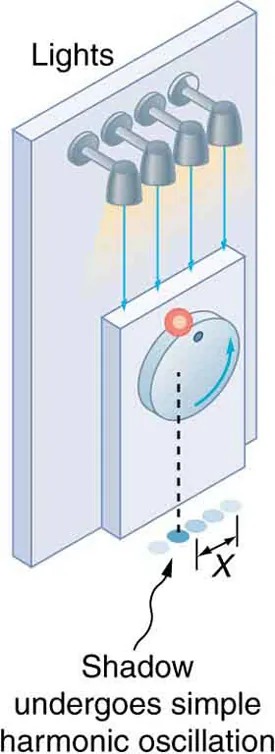
Figure 13.16 The shadow of a ball rotating at constant angular velocity [latex]\omega[/latex] on a turntable goes back and forth in precise simple harmonic motion. Image from OpenStax College Physics 2e, CC-BY 4.0
Image Description
The image depicts a side view of a simple experimental setup demonstrating simple harmonic oscillation. It consists of a fixed wall with a set of five lights mounted on it, shining downwards onto a rotating disk or wheel situated on a lower ledge. The wheel has a marked point highlighted in red, which is shown on the top of the wheel. As the wheel rotates, the shadow of the red point moves back and forth in a linear path on the wall, indicated by a dashed line and labeled ‘X’. This shadow’s movement along the line is described as undergoing simple harmonic oscillation. The image visually explains the relationship between circular motion and simple harmonic motion, as indicated by blue arrows on the rotating wheel and along the shadow path.
Figure 13.17 shows the basic relationship between uniform circular motion and simple harmonic motion. The point P travels around the circle at constant angular velocity [latex]\omega[/latex]. The point P is analogous to an object on the merry-go-round. The projection of the position of P onto a fixed axis undergoes simple harmonic motion and is analogous to the shadow of the object. At the time shown in the figure, the projection has position [latex]x[/latex] and moves to the left with velocity [latex]v[/latex]. The velocity of the point P around the circle equals [latex]\left(\bar{v}\right)_{\text{max}}[/latex].The projection of [latex]\left(\bar{v}\right)_{\text{max}}[/latex] on the [latex]x[/latex]-axis is the velocity [latex]v[/latex] of the simple harmonic motion along the [latex]x[/latex]-axis.
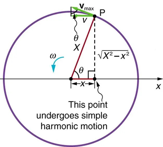
Figure 13.17 A point P moving on a circular path with a constant angular velocity [latex]\omega[/latex] is undergoing uniform circular motion. Its projection on the x-axis undergoes simple harmonic motion. Also shown is the velocity of this point around the circle, [latex]\left(\bar{v}\right)_{\text{max}}[/latex], and its projection, which is [latex]v[/latex]. Note that these velocities form a similar triangle to the displacement triangle. Image from OpenStax College Physics 2e, CC-BY 4.0
Image Description
The image depicts a diagram explaining simple harmonic motion through a circle. The main features are as follows:
- A purple circle with center and radius marked.
- Point P on the circumference of the circle. It is connected to the center by a red line segment, labeled with angle θ and radius X.
- The horizontal axis is labeled x.
- A vertical dashed line drops from point P to intersect the horizontal axis at another point, with the segment labeled √(X² – x²).
- A horizontal segment represents the displacement x.
- Near the center of the circle, there’s an arrow labeled ω, indicating angular velocity.
- The velocity vector v is shown at an angle from point P, with maximum velocity labeled as vmax.
The text states, “This point undergoes simple harmonic motion.”
To see that the projection undergoes simple harmonic motion, note that its position [latex]x[/latex] is given by
[latex]x = X \text{cos} \theta ,[/latex]
where [latex]\theta = \omega t[/latex], [latex]\omega[/latex] is the constant angular velocity, and [latex]X[/latex] is the radius of the circular path. Thus,
[latex]x = X \text{cos} \omega t .[/latex]
The angular velocity [latex]\omega[/latex] is in radians per unit time; in this case [latex]2π[/latex] radians is the time for one revolution [latex]T[/latex]. That is, [latex]\omega = 2π / T[/latex]. Substituting this expression for [latex]\omega[/latex], we see that the position [latex]x[/latex] is given by:
[latex]x \left(\right. t \left.\right) = X \text{cos} \left(\frac{2π t}{T}\right) .[/latex]
This expression is the same one we had for the position of a simple harmonic oscillator in 13.3 Simple Harmonic Motion: A Special Periodic Motion. If we make a graph of position versus time as in Figure 13.18, we see again the wavelike character (typical of simple harmonic motion) of the projection of uniform circular motion onto the [latex]x[/latex]-axis.
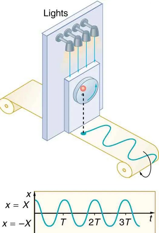
Figure 13.18 The position of the projection of uniform circular motion performs simple harmonic motion, as this wavelike graph of [latex]x[/latex] versus [latex]t[/latex] indicates. Image from OpenStax College Physics 2e, CC-BY 4.0
Image Description
The image consists of two parts: a diagram of a mechanical setup and a graph showing wave patterns.
Mechanical Setup Diagram:
– A vertical panel labeled “Lights” with five attached lamps is depicted.
– Below the lights, a cylindrical device on the panel has a red dot at the top and an arrow pointing upward.
– A flat surface, resembling a paper strip, unwinds from two spools on either side of the panel.
– On this strip, a wavy line is drawn horizontally, indicating a wave traveling across the strip.
Graph of Wave Patterns:
– The graph is divided into sections marked “T,” “2T,” and “3T” along the horizontal axis, labeled as “t.”
– The vertical axis is labeled “x” with points marked as “x = X” at the top and “x = -X” at the bottom.
– A sine wave pattern is shown, with peaks and troughs repeating across the labeled sections.
This illustrates the concept of wave propagation and the role of a mechanical system in generating or analyzing waves.
Now let us use Figure 13.17 to do some further analysis of uniform circular motion as it relates to simple harmonic motion. The triangle formed by the velocities in the figure and the triangle formed by the displacements ([latex]X , x ,[/latex] and [latex]\sqrt{X^{2} - x^{2}}[/latex]) are similar right triangles. Taking ratios of similar sides, we see that
[latex]\frac{v}{v_{\text{max}}} = \frac{\sqrt{X^{2} - x^{2}}}{X} = \sqrt{1 - \frac{x^{2}}{X^{2}}} .[/latex]
We can solve this equation for the speed [latex]v[/latex] or
[latex]v = v_{\text{max}} \sqrt{1 - \frac{x^{2}}{X^{2}}} .[/latex]
This expression for the speed of a simple harmonic oscillator is exactly the same as the equation obtained from conservation of energy considerations in 13.5 Energy and the Simple Harmonic Oscillator. You can begin to see that it is possible to get all of the characteristics of simple harmonic motion from an analysis of the projection of uniform circular motion.
Finally, let us consider the period [latex]T[/latex] of the motion of the projection. This period is the time it takes the point P to complete one revolution. That time is the circumference of the circle [latex]2π X[/latex] divided by the velocity around the circle, [latex]v_{\text{max}}[/latex]. Thus, the period [latex]T[/latex] is
[latex]T = \frac{2πX}{v_{\text{max}}} .[/latex]
We know from conservation of energy considerations that
[latex]v_{\text{max}} = \sqrt{\frac{k}{m}} X .[/latex]
Solving this equation for [latex]X / v_{\text{max}}[/latex] gives
[latex]\frac{X}{v_{\text{max}}} = \sqrt{\frac{m}{k}} .[/latex]
Substituting this expression into the equation for [latex]T[/latex] yields
[latex]T = 2π \sqrt{\frac{m}{k}} .[/latex]
Thus, the period of the motion is the same as for a simple harmonic oscillator. We have determined the period for any simple harmonic oscillator using the relationship between uniform circular motion and simple harmonic motion.
Some modules occasionally refer to the connection between uniform circular motion and simple harmonic motion. Moreover, if you carry your study of physics and its applications to greater depths, you will find this relationship useful. It can, for example, help to analyze how waves add when they are superimposed.
Check Your Understanding
Identify an object that undergoes uniform circular motion. Describe how you could trace the simple harmonic motion of this object as a wave.
Click for Solution
Solution
A record player undergoes uniform circular motion. You could attach dowel rod to one point on the outside edge of the turntable and attach a pen to the other end of the dowel. As the record player turns, the pen will move. You can drag a long piece of paper under the pen, capturing its motion as a wave.
