10.4 Viscosity and Laminar Flow; Poiseuille’s Law
Learning Objectives
By the end of this section, you will be able to:
- Define laminar flow and turbulent flow.
- Explain what viscosity is.
- Calculate flow and resistance with Poiseuille’s law.
- Explain how pressure drops due to resistance.
Laminar Flow and Viscosity
When you pour yourself a glass of juice, the liquid flows freely and quickly. But when you pour syrup on your pancakes, that liquid flows slowly and sticks to the pitcher. The difference is fluid friction, both within the fluid itself and between the fluid and its surroundings. We call this property of fluids viscosity. Juice has low viscosity, whereas syrup has high viscosity. In the previous sections we have considered ideal fluids with little or no viscosity. In this section, we will investigate what factors, including viscosity, affect the rate of fluid flow.
The precise definition of viscosity is based on laminar, or nonturbulent, flow. Before we can define viscosity, then, we need to define laminar flow and turbulent flow. Figure 10.10 shows both types of flow. Laminar flow is characterized by the smooth flow of the fluid in layers that do not mix. Turbulent flow, or turbulence, is characterized by eddies and swirls that mix layers of fluid together.
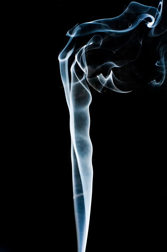
Figure 10.10 Smoke rises smoothly for a while and then begins to form swirls and eddies. The smooth flow is called laminar flow, whereas the swirls and eddies typify turbulent flow. If you watch the smoke (being careful not to breathe on it), you will notice that it rises more rapidly when flowing smoothly than after it becomes turbulent, implying that turbulence poses more resistance to flow. Image from OpenStax College Physics 2e, CC-BY 4.0
Figure 10.11 shows schematically how laminar and turbulent flow differ. Layers flow without mixing when flow is laminar. When there is turbulence, the layers mix, and there are significant velocities in directions other than the overall direction of flow. The lines that are shown in many illustrations are the paths followed by small volumes of fluids. These are called streamlines. Streamlines are smooth and continuous when flow is laminar, but break up and mix when flow is turbulent. Turbulence has two main causes. First, any obstruction or sharp corner, such as in a faucet, creates turbulence by imparting velocities perpendicular to the flow. Second, high speeds cause turbulence. The drag both between adjacent layers of fluid and between the fluid and its surroundings forms swirls and eddies, if the speed is great enough. We shall concentrate on laminar flow for the remainder of this section, leaving certain aspects of turbulence for later sections.
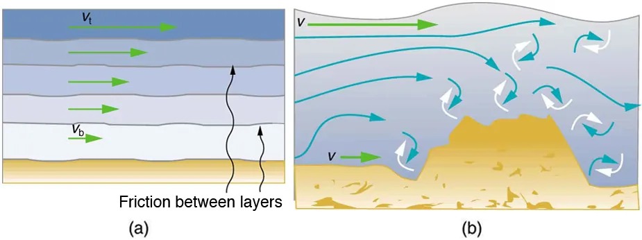
Figure 10.11 (a) Laminar flow occurs in layers without mixing. Notice that viscosity causes drag between layers as well as with the fixed surface. (b) An obstruction in the vessel produces turbulence. Turbulent flow mixes the fluid. There is more interaction, greater heating, and more resistance than in laminar flow. Image from OpenStax College Physics 2e, CC-BY 4.0
Image Description
The image contains two illustrations side by side labeled (a) and (b), depicting fluid dynamics concepts.
Illustration (a): This is a layered fluid flow diagram. It features parallel horizontal layers moving from left to right. The top layer is labeled Vt and the bottom layer is labeled Vb, indicating different velocities. Green arrows illustrate the direction of flow. The phrase “Friction between layers” is pointing to wavy black lines, suggesting interaction or shear between the layers.
Illustration (b): This diagram shows fluid flow over a rough, uneven surface at the bottom. The flow has wavy lines starting at the left and moving towards the right, with green arrows at the beginning of the flow, transitioning to blue arrows as the flow moves over the rough surface. The flow appears to become turbulent, with swirls represented by semicircular arrows, indicating chaotic motion. The bottom of the flow shows a yellow, rough terrain.
Making Connections: Take-Home Experiment: Go Down to the River
Try dropping simultaneously two sticks into a flowing river, one near the edge of the river and one near the middle. Which one travels faster? Why?
Figure 10.12 shows how viscosity is measured for a fluid. Two parallel plates have the specific fluid between them. The bottom plate is held fixed, while the top plate is moved to the right, dragging fluid with it. The layer (or lamina) of fluid in contact with either plate does not move relative to the plate, and so the top layer moves at [latex]v[/latex] while the bottom layer remains at rest. Each successive layer from the top down exerts a force on the one below it, trying to drag it along, producing a continuous variation in speed from [latex]v[/latex] to 0 as shown. Care is taken to insure that the flow is laminar; that is, the layers do not mix. The motion in Figure 10.12 is like a continuous shearing motion. Fluids have zero shear strength, but the rate at which they are sheared is related to the same geometrical factors [latex]A[/latex] and [latex]L[/latex] as is shear deformation for solids.
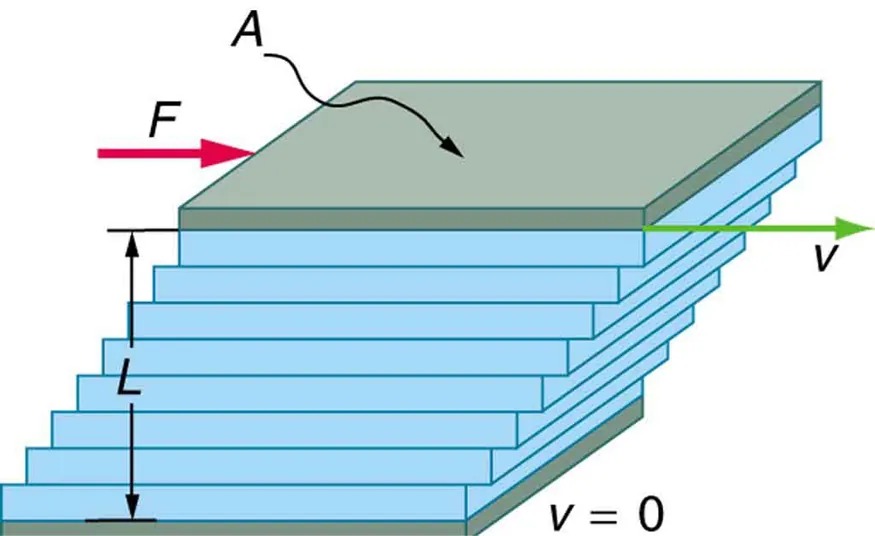
Figure 10.12 The graphic shows laminar flow of fluid between two plates of area [latex]A[/latex]. The bottom plate is fixed. When the top plate is pushed to the right, it drags the fluid along with it. Image from OpenStax College Physics 2e, CC-BY 4.0
Image Description
The image depicts a diagram illustrating the concept of shear stress in a fluid. It shows a stack of horizontal layers that represent fluid sheets, with each one sliding over the one below it. At the top, there is a rectangular block labeled “A.” An arrow labeled “F” points to the right, indicating a force applied to the top layer. Another arrow labeled “v” points horizontally to the right, indicating the velocity of fluid layers in that direction. The bottom layer is grounded with a label “v = 0,” indicating no velocity. A vertical arrow labeled “L” points downward on the left side, possibly indicating the thickness or distance between layers. The entire setup shows fluid motion under the influence of an applied force, demonstrating how different layers can move at various speeds due to the force exerted on them.
A force [latex]F[/latex] is required to keep the top plate in Figure 10.12 moving at a constant velocity [latex]v[/latex], and experiments have shown that this force depends on four factors. First, [latex]F[/latex] is directly proportional to [latex]v[/latex] (until the speed is so high that turbulence occurs—then a much larger force is needed, and it has a more complicated dependence on [latex]v[/latex]). Second, [latex]F[/latex] is proportional to the area [latex]A[/latex] of the plate. This relationship seems reasonable, since [latex]A[/latex] is directly proportional to the amount of fluid being moved. Third, [latex]F[/latex] is inversely proportional to the distance between the plates [latex]L[/latex]. This relationship is also reasonable; [latex]L[/latex] is like a lever arm, and the greater the lever arm, the less force that is needed. Fourth, [latex]F[/latex] is directly proportional to the coefficient of viscosity, [latex]\eta[/latex]. The greater the viscosity, the greater the force required. These dependencies are combined into the equation
[latex]F = \eta \frac{\text{vA}}{L} ,[/latex]
which gives us a working definition of fluid viscosity [latex]\eta[/latex]. Solving for [latex]\eta[/latex] gives
[latex]\eta = \frac{\text{FL}}{\text{vA}} ,[/latex]
which defines viscosity in terms of how it is measured. The SI unit of viscosity is [latex]\text{N} \cdot \text{m}/ \left[\right. \left(\right. \text{m}/\text{s} \left.\right) \text{m}^{2} \left]\right. = \left(\right. \text{N}/\text{m}^{2} \left.\right) \text{s or Pa} \cdot \text{s}[/latex]. Table 10.1 lists the coefficients of viscosity for various fluids.
Viscosity varies from one fluid to another by several orders of magnitude. As you might expect, the viscosities of gases are much less than those of liquids, and these viscosities are often temperature dependent. The viscosity of blood can be reduced by aspirin consumption, allowing it to flow more easily around the body. (When used over the long term in low doses, aspirin can help prevent heart attacks, and reduce the risk of blood clotting.)
Laminar Flow Confined to Tubes—Poiseuille’s Law
What causes flow? The answer, not surprisingly, is pressure difference. In fact, there is a very simple relationship between horizontal flow and pressure. Flow rate [latex]Q[/latex] is in the direction from high to low pressure. The greater the pressure differential between two points, the greater the flow rate. This relationship can be stated as
[latex]Q = \frac{P_{2} - P_{1}}{R} ,[/latex]
where [latex]P_{1}[/latex] and [latex]P_{2}[/latex] are the pressures at two points, such as at either end of a tube, and [latex]R[/latex] is the resistance to flow. The resistance [latex]R[/latex] includes everything, except pressure, that affects flow rate. For example, [latex]R[/latex] is greater for a long tube than for a short one. The greater the viscosity of a fluid, the greater the value of [latex]R[/latex]. Turbulence greatly increases [latex]R[/latex], whereas increasing the diameter of a tube decreases [latex]R[/latex].
If viscosity is zero, the fluid is frictionless and the resistance to flow is also zero. Comparing frictionless flow in a tube to viscous flow, as in Figure 10.13, we see that for a viscous fluid, speed is greatest at midstream because of drag at the boundaries. We can see the effect of viscosity in a Bunsen burner flame, even though the viscosity of natural gas is small.
The resistance [latex]R[/latex] to laminar flow of an incompressible fluid having viscosity [latex]\eta[/latex] through a horizontal tube of uniform radius [latex]r[/latex] and length [latex]l[/latex], such as the one in Figure 10.14, is given by
[latex]R = \frac{8 \eta l}{\pi r^{4}} .[/latex]
This equation is called Poiseuille’s law for resistance after the French scientist J. L. Poiseuille (1799–1869), who derived it in an attempt to understand the flow of blood, an often turbulent fluid.
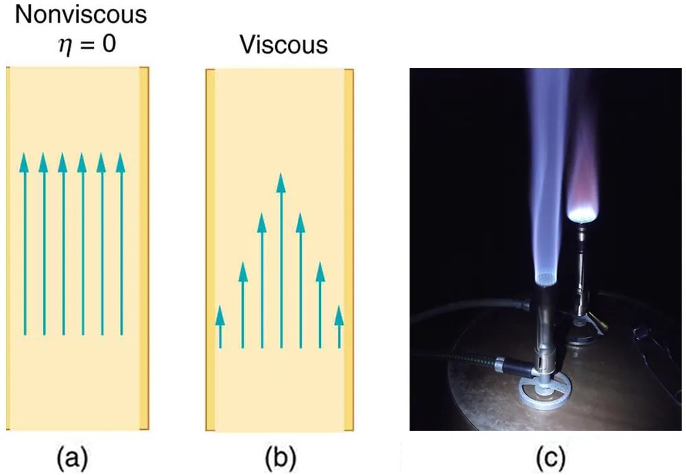
Figure 10.13 (a) If fluid flow in a tube has negligible resistance, the speed is the same all across the tube. (b) When a viscous fluid flows through a tube, its speed at the walls is zero, increasing steadily to its maximum at the center of the tube. (c) The shape of the Bunsen burner flame is due to the velocity profile across the tube. Image from OpenStax College Physics 2e, CC-BY 4.0
Image Description
The image contains three parts labeled (a), (b), and (c).
Part (a): A diagram titled “Nonviscous η = 0” featuring a rectangular section with straight, vertical lines representing flow paths. The lines are evenly spaced and parallel, indicating a uniform flow with no viscosity.
Part (b): A diagram titled “Viscous” showing a similar rectangular section, but with curved lines representing flow paths. The lines are wider at the edges and curved toward the center, illustrating how viscosity causes variation in flow speed, with faster flow in the center.
Part (c): A photograph showing a flame produced by a Bunsen burner in a dark environment. The flame is bright at the base and tapers off to a faint bluish color as it ascends, indicating gas combustion under laboratory conditions.
Let us examine Poiseuille’s expression for [latex]R[/latex] to see if it makes good intuitive sense. We see that resistance is directly proportional to both fluid viscosity [latex]\eta[/latex] and the length [latex]l[/latex] of a tube. After all, both of these directly affect the amount of friction encountered—the greater either is, the greater the resistance and the smaller the flow. The radius [latex]r[/latex] of a tube affects the resistance, which again makes sense, because the greater the radius, the greater the flow (all other factors remaining the same). But it is surprising that [latex]r[/latex] is raised to the fourth power in Poiseuille’s law. This exponent means that any change in the radius of a tube has a very large effect on resistance. For example, doubling the radius of a tube decreases resistance by a factor of [latex]2^{4} = \text{16}[/latex].
Taken together, [latex]Q = \frac{P_{2} - P_{1}}{R}[/latex] and [latex]R = \frac{8 \eta l}{\pi r^{4}}[/latex] give the following expression for flow rate:
[latex]Q = \frac{\left(\right. P_{2} - P_{1} \left.\right) πr^{4}}{8 \eta l} .[/latex]
This equation describes laminar flow through a tube. It is sometimes called Poiseuille’s law for laminar flow, or simply Poiseuille’s law.
Example 10.7
Using Flow Rate: Plaque Deposits Reduce Blood Flow
Suppose the flow rate of blood in a coronary artery has been reduced to half its normal value by plaque deposits. By what factor has the radius of the artery been reduced, assuming no turbulence occurs?
Strategy
Assuming laminar flow, Poiseuille’s law states that
[latex]Q = \frac{\left(\right. P_{2} - P_{1} \left.\right) πr^{4}}{8 \eta l} .[/latex]
We need to compare the artery radius before and after the flow rate reduction.
Solution
With a constant pressure difference assumed and the same length and viscosity, along the artery we have
[latex]\frac{Q_{1}}{r_{1}^{4}} = \frac{Q_{2}}{r_{2}^{4}} .[/latex]
So, given that [latex]Q_{2} = 0 . \text{5} Q_{1}[/latex], we find that [latex]r_{2}^{4} = 0 . \left(5 r\right)_{1}^{4}[/latex].
Therefore, [latex]r_{2} = \left(0 . 5\right)^{0 . \text{25}} r_{1} = 0 . \text{841} r_{1}[/latex], a decrease in the artery radius of 16%.
Discussion
This decrease in radius is surprisingly small for this situation. To restore the blood flow in spite of this buildup would require an increase in the pressure difference [latex]\left(P_{2} - P_{1}\right)[/latex] of a factor of two, with subsequent strain on the heart.
| Fluid | Temperature (ºC) | Viscosity [latex]\eta (\text{mPa}\cdot\text{s})[/latex] |
|---|---|---|
| Gases | ||
| Air | 0 | 0.0171 |
| 20 | 0.0181 | |
| 40 | 0.0190 | |
| 100 | 0.0218 | |
| Ammonia | 20 | 0.00974 |
| Carbon dioxide | 20 | 0.0147 |
| Helium | 20 | 0.0196 |
| Hydrogen | 0 | 0.0090 |
| Mercury | 20 | 0.0450 |
| Oxygen | 20 | 0.0203 |
| Steam | 100 | 0.0130 |
| Liquids | ||
| Water | 0 | 1.792 |
| 20 | 1.002 | |
| 37 | 0.6947 | |
| 40 | 0.653 | |
| 100 | 0.282 | |
| Whole blood[1] | 20 | 3.015 |
| 37 | 2.084 | |
| Blood plasma[2] | 20 | 1.810 |
| 37 | 1.257 | |
| Ethyl alcohol | 20 | 1.20 |
| Methanol | 20 | 0.584 |
| Oil (heavy machine) | 20 | 660 |
| Oil (motor, SAE 10) | 30 | 200 |
| Oil (olive) | 20 | 138 |
| Glycerin | 20 | 1500 |
| Honey | 20 | 2000–10000 |
| Maple Syrup | 20 | 2000–3000 |
| Milk | 20 | 3.0 |
| Oil (Corn) | 20 | 65 |
The circulatory system provides many examples of Poiseuille’s law in action—with blood flow regulated by changes in vessel size and blood pressure. Blood vessels are not rigid but elastic. Adjustments to blood flow are primarily made by varying the size of the vessels, since the resistance is so sensitive to the radius. During vigorous exercise, blood vessels are selectively dilated to important muscles and organs and blood pressure increases. This creates both greater overall blood flow and increased flow to specific areas. Conversely, decreases in vessel radii, perhaps from plaques in the arteries, can greatly reduce blood flow. If a vessel’s radius is reduced by only 5% (to 0.95 of its original value), the flow rate is reduced to about [latex]\left(\right. 0 . \text{95} \left.\right)^{4} = 0 . \text{81}[/latex] of its original value. A 19% decrease in flow is caused by a 5% decrease in radius. The body may compensate by increasing blood pressure by 19%, but this presents hazards to the heart and any vessel that has weakened walls. Another example comes from automobile engine oil. If you have a car with an oil pressure gauge, you may notice that oil pressure is high when the engine is cold. Motor oil has greater viscosity when cold than when warm, and so pressure must be greater to pump the same amount of cold oil.
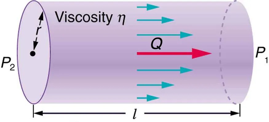
Figure 10.14 Poiseuille’s law applies to laminar flow of an incompressible fluid of viscosity [latex]\eta[/latex] through a tube of length [latex]l[/latex] and radius [latex]r[/latex]. The direction of flow is from greater to lower pressure. Flow rate [latex]Q[/latex] is directly proportional to the pressure difference [latex]P_{2} - P_{1}[/latex], and inversely proportional to the length [latex]l[/latex] of the tube and viscosity [latex]\eta[/latex] of the fluid. Flow rate increases with [latex]r^{4}[/latex], the fourth power of the radius. Image from OpenStax College Physics 2e, CC-BY 4.0
Image Description
The image illustrates fluid flow through a cylindrical pipe, representing concepts in fluid dynamics. The cylinder is shown as a long, purple tube with its length extending horizontally. At the left end of the cylinder, the pressure is labeled as P2, and at the right end, it’s labeled as P1. The flow direction is from right to left, indicating that P1 is greater than P2.
Inside the cylinder, multiple arrows of varying lengths are drawn parallel to the axis, pointing in the flow direction. A larger red arrow labeled as Q represents the overall flow rate, while smaller blue arrows illustrate velocity distribution across the pipe’s cross-section.
The viscosity of the fluid is noted by the Greek letter eta (η). The radius of the pipe is marked with a line and labeled as r, starting from the center to the wall of the cylinder. The length of the pipe is denoted as l, spanning from one end to the other.
Example 10.8
What Pressure Produces This Flow Rate?
An intravenous (IV) system is supplying saline solution to a patient at the rate of [latex]0 . \text{120} \text{cm}^{3} /\text{s}[/latex] through a needle of radius 0.150 mm and length 2.50 cm. What pressure is needed at the entrance of the needle to cause this flow, assuming the viscosity of the saline solution to be the same as that of water? The gauge pressure of the blood in the patient’s vein is 8.00 mm Hg. (Assume that the temperature is [latex]\text{20}º\text{C}[/latex].)
Strategy
Assuming laminar flow, Poiseuille’s law applies. This is given by
[latex]Q = \frac{\left(\right. P_{2} - P_{1} \left.\right) \pi r^{4}}{8 \eta l} ,[/latex]
where [latex]P_{2}[/latex] is the pressure at the entrance of the needle and [latex]P_{1}[/latex] is the pressure in the vein. The only unknown is [latex]P_{2}[/latex].
Solution
Solving for [latex]P_{2}[/latex] yields
[latex]P_{2} = \frac{8 \eta l}{πr^{4}} Q + P_{1 .}[/latex]
[latex]P_{1}[/latex] is given as 8.00 mm Hg, which converts to [latex]1 . \text{066} \times \text{10}^{3} \text{N}/\text{m}^{2}[/latex]. Substituting this and the other known values yields
[latex]{\small\begin{eqnarray*}P_{2} & = & \left[\frac{8 \left(\right. 1 . \text{00} \times \text{10}^{- 3} \text{N} \cdot \text{s}/\text{m}^{2} \left.\right) \left(\right. 2 . \text{50} \times \text{10}^{- 2} \text{m} \left.\right)}{\pi \left(\right. 0 . \text{150} \times \text{10}^{- 3} \text{m} \left.\right)^{4}}\right]\\ & \text{ } &\;\;\;\times \left(\right. 1 . \text{20} \times \text{10}^{- 7} \text{m}^{3} /\text{s} \left.\right) + 1 . \text{066} \times \text{10}^{3} \text{N}/\text{m}^{2} \\[1.5ex] & = & 1 . \text{62} \times \text{10}^{4} \text{N}/\text{m}^{2} .\end{eqnarray*}}[/latex]
Discussion
This pressure could be supplied by an IV bottle with the surface of the saline solution 1.61 m above the entrance to the needle (this is left for you to solve in this chapter’s Problems and Exercises), assuming that there is negligible pressure drop in the tubing leading to the needle.
Flow and Resistance as Causes of Pressure Drops
You may have noticed that water pressure in your home might be lower than normal on hot summer days when there is more use. This pressure drop occurs in the water main before it reaches your home. Let us consider flow through the water main as illustrated in Figure 10.15. We can understand why the pressure [latex]P_{1}[/latex] to the home drops during times of heavy use by rearranging
[latex]Q = \frac{P_{2} - P_{1}}{R}[/latex]
to
[latex]P_{2} - P_{1} = R Q ,[/latex]
where, in this case, [latex]P_{2}[/latex] is the pressure at the water works and [latex]R[/latex] is the resistance of the water main. During times of heavy use, the flow rate [latex]Q[/latex] is large. This means that [latex]P_{2} - P_{1}[/latex] must also be large. Thus [latex]P_{1}[/latex] must decrease. It is correct to think of flow and resistance as causing the pressure to drop from [latex]P_{2}[/latex] to [latex]P_{1}[/latex]. [latex]P_{2} - P_{1} = R Q[/latex] is valid for both laminar and turbulent flows.
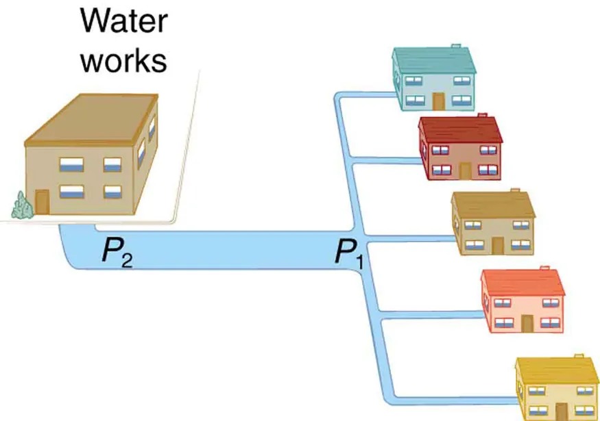
Figure 10.15 During times of heavy use, there is a significant pressure drop in a water main, and [latex]P_{\text{1}}[/latex] supplied to users is significantly less than[latex]P_{\text{2}}[/latex] created at the water works. If the flow is very small, then the pressure drop is negligible, and [latex]P_{2} \approx P_{1}[/latex]. Image from OpenStax College Physics 2e, CC-BY 4.0
Image Description
The image depicts a simplified diagram of a water distribution system. On the left, there is a large building labeled “Water works,” representing the water supply center. From this building, a main pipe extends to the right, labeled “P2,” which then splits into several smaller pipes labeled “P1.” These smaller pipes branch out to connect to several houses on the right side of the image. There are six houses in total, each of a different color: teal, red, brown, orange, and yellow. The houses are arranged in two rows, with three on the top and three on the bottom. The pipes are illustrated in blue, and the system shows how water is distributed from the water works to the individual houses.
We can use [latex]P_{2} - P_{1} = R Q[/latex] to analyze pressure drops occurring in more complex systems in which the tube radius is not the same everywhere. Resistance will be much greater in narrow places, such as an obstructed coronary artery. For a given flow rate [latex]Q[/latex], the pressure drop will be greatest where the tube is most narrow. This is how water faucets control flow. Additionally, [latex]R[/latex] is greatly increased by turbulence, and a constriction that creates turbulence greatly reduces the pressure downstream. Plaque in an artery reduces pressure and hence flow, both by its resistance and by the turbulence it creates.
Figure 10.16 is a schematic of the human circulatory system, showing average blood pressures in its major parts for an adult at rest. Pressure created by the heart’s two pumps, the right and left ventricles, is reduced by the resistance of the blood vessels as the blood flows through them. The left ventricle increases arterial blood pressure that drives the flow of blood through all parts of the body except the lungs. The right ventricle receives the lower pressure blood from two major veins and pumps it through the lungs for gas exchange with atmospheric gases – the disposal of carbon dioxide from the blood and the replenishment of oxygen. Only one major organ is shown schematically, with typical branching of arteries to ever smaller vessels, the smallest of which are the capillaries, and rejoining of small veins into larger ones. Similar branching takes place in a variety of organs in the body, and the circulatory system has considerable flexibility in flow regulation to these organs by the dilation and constriction of the arteries leading to them and the capillaries within them. The sensitivity of flow to tube radius makes this flexibility possible over a large range of flow rates.
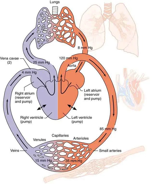
Figure 10.16 Schematic of the circulatory system. Pressure difference is created by the two pumps in the heart and is reduced by resistance in the vessels. Branching of vessels into capillaries allows blood to reach individual cells and exchange substances, such as oxygen and waste products, with them. The system has an impressive ability to regulate flow to individual organs, accomplished largely by varying vessel diameters. Image from OpenStax College Physics 2e, CC-BY 4.0
Image Description
This image is a diagram of the human circulatory system, illustrating the flow of blood through the heart, lungs, and the body. It is divided into two sides: the left side (depicted in red) and the right side (depicted in blue).
The left side of the heart collects oxygen-rich blood from the lungs and pumps it to the body, while the right side collects deoxygenated blood from the body and pumps it to the lungs for oxygenation.
The system is labeled with various components and blood pressures at different points:
- Lungs: Shown above the heart.
- Arteries: Highlighted in red, carrying blood away from the heart.
- Veins: Highlighted in blue, carrying blood to the heart.
- Right Atrium: Acts as a reservoir and pump, receiving deoxygenated blood from the body.
- Right Ventricle: Pumps deoxygenated blood to the lungs.
- Left Atrium: Acts as a reservoir and pump, receiving oxygenated blood from the lungs.
- Left Ventricle: Pumps oxygenated blood to the body.
- Vena Cavae: Two large veins bringing deoxygenated blood back to the heart, labeled with a pressure of 2 and 25 mm Hg.
- Aorta: The main artery, labeled with a pressure of 120 mm Hg.
- Arterioles and Small Arteries: Also highlighted in red, leading to capillaries, with pressures labeled at 85 mm Hg.
- Capillaries: Network where oxygen and nutrients are exchanged, with pressures labeled at 35 mm Hg.
- Venules: Small veins leading from capillaries, labeled with a pressure of 15 mm Hg.
The diagram visually represents how blood circulates through this closed-loop system, emphasizing the differences between oxygenated and deoxygenated pathways and their associated pressures.
Each branching of larger vessels into smaller vessels increases the total cross-sectional area of the tubes through which the blood flows. For example, an artery with a cross section of [latex]1 \text{cm}^{2}[/latex] may branch into 20 smaller arteries, each with cross sections of [latex]0.5 \text{cm}^{2}[/latex], with a total of [latex]\text{10} \text{cm}^{2}[/latex]. In that manner, the resistance of the branchings is reduced so that pressure is not entirely lost. Moreover, because [latex]Q = A \bar{v}[/latex] and [latex]A[/latex] increases through branching, the average velocity of the blood in the smaller vessels is reduced. The blood velocity in the aorta ([latex]\text{diameter} = 1 \text{cm}[/latex]) is about 25 cm/s, while in the capillaries ([latex]\text{20 } \mu \text{m}[/latex] in diameter) the velocity is about 1 mm/s. This reduced velocity allows the blood to exchange substances with the cells in the capillaries and alveoli in particular.
