28
Ma trận đối xứng và hàm bậc hai
Ma trận đối xứng
Một ma trận vuông \(A \in \mathbb{R}^{n\times n}\) là đối xứng nếu nó bằng với ma trận chuyển vị của nó. Tức là,
[latex]\begin{equation*} A_{ij} = A_{ji}, \quad 1 \leq i,j \leq n. \end{equation*}[/latex]
Tập hợp các ma trận đối xứng \(n \times n\) được ký hiệu là \({\bf S}^n\). Tập hợp này là một không gian con của \(\mathbb{R}^{n\times n}\).
| Ví dụ 1: Ma trận đối xứng \(3 \times 3\). |
| Ma trận |
| \[ A = \begin{pmatrix} 4 & 3/2 & 2 \\ 3/2 & 2 & 5/2 \\ 2 & 5/2 & 2 \end{pmatrix} \] |
| là đối xứng. Ma trận |
| \[ A = \begin{pmatrix} 4 & 3/2 & 2 \\ 3/2 & 2 & \mathbf{5} \\ 2 & \mathbf{5/2} & 2 \end{pmatrix} \] |
|
thì không đối xứng, vì nó không bằng với ma trận chuyển vị của nó.
|
Xem thêm:
- Biểu diễn của một đồ thị vô hướng có trọng số.
- Ma trận Laplace của một đồ thị.
- Ma trận Hess của một hàm số.
- Ma trận Gram của các điểm dữ liệu.
Hàm bậc hai
Một hàm \(q: \mathbb{R}^n \rightarrow \mathbb{R}\) được gọi là một hàm bậc hai nếu nó có thể được biểu diễn dưới dạng
[latex]\begin{align*} q(x) &= \sum\limits_{i=1}^n \sum\limits_{j=1}^n A_{ij}x_ix_j+2\sum\limits_{i=1}^n b_ix_i+c, \end{align*}[/latex]
với các số \(A_{ij}, b_i\), và \(c, i,j \in \{1,\cdots,n\}\). Một hàm bậc hai do đó là một tổ hợp afin của các biến \(x_i\) và tất cả các "tích chéo" \(x_i x_j\). Ta quan sát thấy hệ số của \(x_i x_j\) là \((A_{ij} + A_{ji})\).
Hàm này được gọi là một dạng toàn phương nếu không có các số hạng tuyến tính hoặc hằng số trong đó:
[latex]\begin{equation*} b_i = 0, \quad c_i = 0. \end{equation*}[/latex]
Lưu ý rằng ma trận Hess (ma trận của các đạo hàm cấp hai) của một hàm bậc hai là một hằng số.
Ví dụ:
Mối liên hệ giữa hàm bậc hai và ma trận đối xứng
Có một mối quan hệ tự nhiên giữa ma trận đối xứng và hàm bậc hai. Thật vậy, bất kỳ hàm bậc hai \(q: \mathbb{R}^n \rightarrow \mathbb{R}\) nào cũng có thể được viết dưới dạng
[latex]\begin{equation*} q(x) = \begin{pmatrix} x \\ 1 \end{pmatrix}^T\begin{pmatrix} A & b \\ b^T & c \end{pmatrix}\begin{pmatrix} x \\ 1 \end{pmatrix} = x^T A x + 2 b^T x + c \end{equation*}[/latex]
với một ma trận đối xứng \(A \in {\bf S}^n\) thích hợp, véctơ \(b \in \mathbb{R}^n\) và vô hướng \(c \in \mathbb{R}\). Ở đây:
- [latex]A_{ii}[/latex] là hệ số của [latex]x_i^2[/latex] trong [latex]q[/latex];
- với [latex]i \neq j[/latex], [latex]2A_{ij}[/latex] là hệ số của số hạng [latex]x_i x_j[/latex] trong [latex]q[/latex];
- [latex]2b_i[/latex] là hệ số của số hạng [latex]x_i[/latex];
- [latex]c[/latex] là số hạng hằng, [latex]q(0)[/latex].
Nếu [latex]q[/latex] là một dạng toàn phương, thì [latex]b=0[/latex], [latex]c=0[/latex], và ta có thể viết [latex]q(x) = x^TAx[/latex] trong đó [latex]A \in {\bf S}^n[/latex].
Ví dụ: Ví dụ trong trường hợp hai chiều.
28.2. Xấp xỉ bậc hai của các hàm phi tuyến
Ta đã thấy các hàm tuyến tính phát sinh như thế nào khi tìm một xấp xỉ tuyến tính đơn giản cho một hàm phi tuyến phức tạp hơn. Tương tự, các hàm bậc hai phát sinh một cách tự nhiên khi ta tìm cách xấp xỉ một hàm phi tuyến cho trước bằng một hàm bậc hai.
Trường hợp một chiều
Nếu [latex]f: \mathbb{R} \rightarrow \mathbb{R}[/latex] là một hàm khả vi hai lần thì xấp xỉ bậc hai (hay, khai triển Taylor bậc hai) của [latex]f[/latex] tại một điểm [latex]x_0[/latex] có dạng
[latex]\begin{align*} f(x) &\approx q(x) = f(x_0)+f'(x_0)(x-x_0)+\frac{1}{2}f''(x_0)(x-x_0)^2, \end{align*}[/latex]
trong đó [latex]f'(x_0)[/latex] là đạo hàm cấp một, và [latex]f''(x_0)[/latex] là đạo hàm cấp hai của [latex]f[/latex] tại [latex]x_0[/latex]. Ta quan sát thấy xấp xỉ bậc hai [latex]q[/latex] có cùng giá trị, đạo hàm, và đạo hàm cấp hai như [latex]f[/latex], tại [latex]x_0[/latex].
 |
|
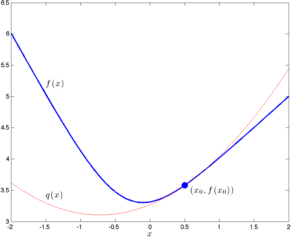
| Ví dụ 2: Hình vẽ cho thấy một xấp xỉ bậc hai [latex]q[/latex] của hàm một biến [latex]f:\mathbb{R} \rightarrow \mathbb{R}[/latex], với các giá trị | |
| [latex]\begin{align*} f(x) &= \log(\exp(x-3)+\exp(-2x+2)), \end{align*}[/latex] | |
| tại điểm [latex]x_0 = 0.5[/latex] (màu đỏ). | |
Trường hợp nhiều chiều
Trong nhiều chiều, ta có một kết quả tương tự. Ta hãy xấp xỉ một hàm khả vi hai lần [latex]f: \mathbb{R}^n \rightarrow \mathbb{R}[/latex] bằng một hàm bậc hai [latex]q[/latex], sao cho [latex]f[/latex] và [latex]q[/latex] trùng nhau cho đến đạo hàm cấp hai.
Hàm [latex]q[/latex] phải có dạng
[latex]\begin{align*} q(x) &= x^TAx+2b^Tx+c, \end{align*}[/latex]
trong đó [latex]A \in {\bf S}^n[/latex], [latex]b \in \mathbb{R}^n[/latex], và [latex]c \in \mathbb{R}[/latex]. Điều kiện của ta rằng [latex]q[/latex] trùng với [latex]f[/latex] cho đến đạo hàm cấp hai cho thấy ta phải có
[latex]\begin{align*} \nabla^2 q(x) &= 2A = \nabla^2 f(x_0), \\ \nabla q(x) &= 2(Ax_0+b) = \nabla f(x_0), \\ x^TAx_0 + 2b^Tx_0 + c &= f(x_0), \end{align*}[/latex]
trong đó [latex]\nabla^2 f(x_0)[/latex] là ma trận Hesse, và [latex]\nabla f(x_0)[/latex] là gradient, của [latex]f[/latex] tại [latex]x_0[/latex].
Giải tìm [latex]A,b,c[/latex] ta thu được kết quả sau:
Khai triển bậc hai của một hàm số: Xấp xỉ bậc hai của một hàm khả vi hai lần [latex]f[/latex] tại một điểm [latex]x_0[/latex] có dạng
[latex]\begin{align*} f(x) &\approx q(x) = f(x_0)+\nabla f(x_0)^T(x-x_0)+\frac{1}{2}(x-x_0)^T\nabla^2 f(x_0)(x-x_0), \end{align*}[/latex]
trong đó [latex]\nabla f(x_0) \in \mathbb{R}^n[/latex] là gradient của [latex]f[/latex] tại [latex]x_0[/latex], và ma trận đối xứng [latex]\nabla^2 f(x_0)[/latex] là ma trận Hess của [latex]f[/latex] tại [latex]x_0[/latex].
Ví dụ: Khai triển bậc hai của hàm log-sum-exp.
28.3. Các ma trận đối xứng đặc biệt
Ma trận đường chéo
Trường hợp đặc biệt đơn giản nhất của ma trận đối xứng là lớp các ma trận đường chéo, vốn chỉ có các phần tử khác không trên đường chéo.
Nếu [latex]\lambda \in \mathbb{R}^n[/latex], ta ký hiệu [latex]{\bf diag}(\lambda_1, \cdots, \lambda_n)[/latex], hay viết tắt là [latex]{\bf diag} (\lambda)[/latex], là ma trận đường chéo (đối xứng) [latex]n \times n[/latex] với [latex]\lambda[/latex] trên đường chéo của nó. Ma trận đường chéo tương ứng với các dạng toàn phương có dạng
[latex]\begin{align*} q(x) &= \sum\limits_{i=1}^n \lambda_i x_i^2 = x^T{\bf diag}(\lambda)x. \end{align*}[/latex]
Các hàm như vậy không có bất kỳ "số hạng chéo" nào có dạng [latex]x_i x_j[/latex] với [latex]i \neq j[/latex].
| Ví dụ 3: Một ma trận đường chéo và dạng toàn phương tương ứng của nó.
Định nghĩa một ma trận đường chéo: [latex]\begin{align*} D &:= \mathbf{diag}(1,4,-3) =\begin{pmatrix} 1 & 0 & 0 \\ 0 & 4 & 0 \\ 0 & 0 & -3 \end{pmatrix}. \end{align*}[/latex] Với ma trận trên, dạng toàn phương tương ứng là [latex]\begin{align*} q(x) &= x^T\begin{pmatrix} 1 & 0 & 0 \\ 0 & 4 & 0 \\ 0 & 0 & -3 \end{pmatrix} x = x_1^2 +4x_2^2 - 3x_3^2. \end{align*}[/latex] |
Dyad đối xứng
Một lớp các ma trận đối xứng quan trọng khác đó là các ma trận có dạng [latex]uu^T[/latex], trong đó [latex]u \in \mathbb{R}^n[/latex]. Ma trận này có các phần tử là [latex]u_i u_j[/latex] và là ma trận đối xứng. Các ma trận như vậy được gọi là dyad đối xứng. (Nếu [latex]||u||_2=1[/latex], thì dyad được gọi là dyad chuẩn hóa.)
Dyad đối xứng tương ứng với các dạng toàn phương chỉ đơn giản là các dạng tuyến tính bình phương: [latex]q(x) = (u^Tx)^2[/latex].
Ví dụ: Dạng tuyến tính bình phương.
