16
16.1 Mô hình không gian trạng thái của các hệ động lực tuyến tính.
Định nghĩa
Rất nhiều hệ động lực thời gian rời rạc có thể được mô hình hóa thông qua các phương trình không gian trạng thái tuyến tính, có dạng
\[x(t+1)=Ax(t)+Bu(t), \quad y(t)=Cx(t)+Du(t), \quad t=0,1,2,\dots\]
trong đó \(x(t) \in \mathbb{R}^{n}\) là trạng thái, bao hàm trạng thái của hệ tại thời điểm \(t, u(t) \in \mathbb{R}^{p}\) chứa các biến điều khiển, \(y(t) \in \mathbb{R}^{k}\) chứa các đầu. Các ma trận
\[ A \in \mathbb{R}^{n \times n}, \quad B \in \mathbb{R}^{n \times p}, \quad C \in \mathbb{R}^{k \times n}, \quad D \in \mathbb{R}^{k \times p} \]
có cỡ phù hợp để đảm bảo tính tương thích của các phép nhân ma trận.
Thực chất, một mô hình động lực tuyến tính phát biểu rằng trạng thái tại thời điểm kế tiếp là một hàm tuyến tính của trạng thái tại các thời điểm trước đó, và có thể cả các đầu vào ‘‘ngoại sinh’’ khác; và rằng đầu ra là một hàm tuyến tính của véctơ trạng thái và véctơ đầu vào.
Một mô hình thời gian liên tục sẽ có dạng một phương trình vi phân
\[\dfrac{d}{dt}x(t)=Ax(t)+Bu(t), \quad y(t)=Cx(t)+Du(t), \quad t \ge 0.\]
Cuối cùng, các mô hình cái gọi là biến thiên theo thời gian bao gồm các ma trận \(A, B, C, D\) biến thiên theo thời gian (xem một ví dụ bên dưới).
Bài toán mở đầu
Động lực chính của mô hình không gian trạng thái là khả năng mô hình hóa các đạo hàm bậc cao trong các phương trình động lực, chỉ bằng cách sử dụng các đạo hàm bậc nhất, nhưng dùng véctơ thay vì các đại lượng vô hướng.
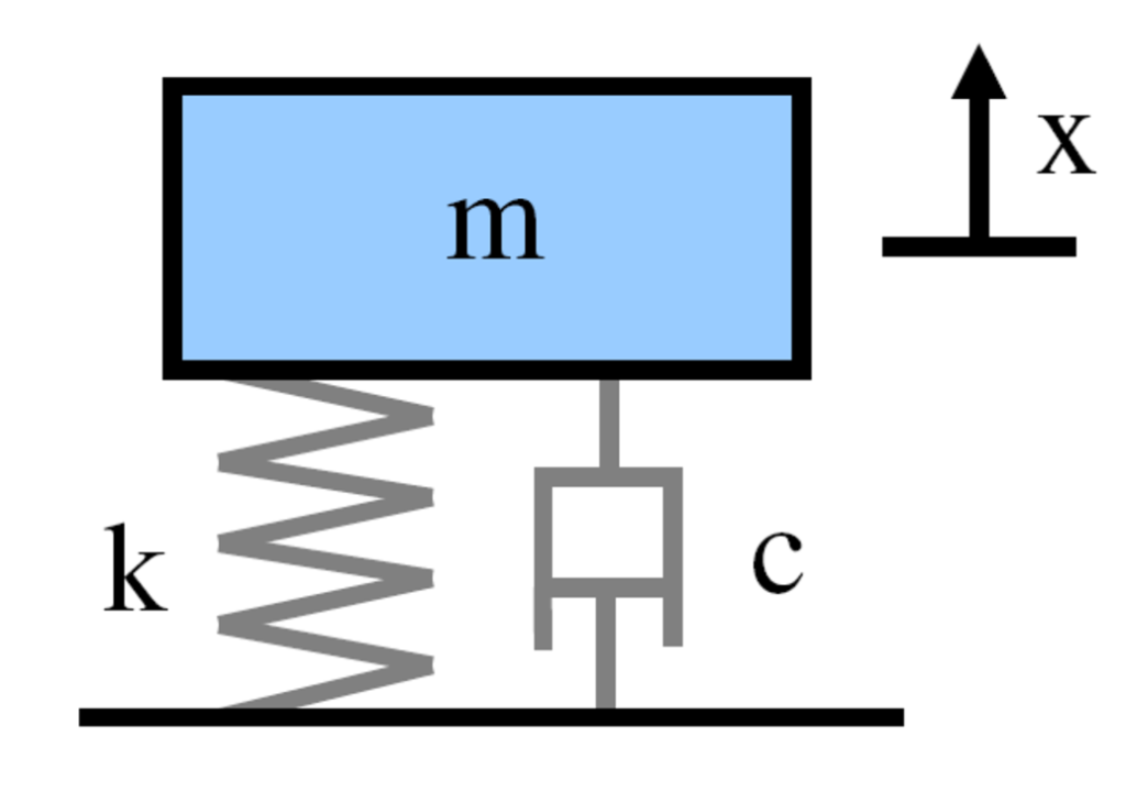 |
Chẳng hạn, xét phương trình vi phân bậc hai:
\[ m\ddot{y}(t) + c\dot{y}(t) + ky(t) = u(t) \] mô tả động lực học của một hệ lò xo-khối lượng có giảm chấn. Trong phương trình này: \( m \) : khối lượng của vật gắn vào lò xo. \( c \) : hệ số giảm chấn. \( k \) : hằng số lò xo. \( u(t) \) : ngoại lực bất kỳ tác động lên khối lượng. \( y(t) \) : độ dời theo phương thẳng đứng của khối lượng so với vị trí cân bằng. |
Phương trình trên chứa đạo hàm bậc hai của một hàm vô hướng \(y(\cdot)\). Chúng ta có thể biểu diễn nó dưới dạng tương đương chỉ chứa các đạo hàm bậc nhất, bằng cách định nghĩa véctơ trạng thái là
\[x(t) := \begin{pmatrix} y(t) \\ \dot{y}(t) \end{pmatrix}.\]
Bây giờ chúng ta xử lý một phương trình véctơ thay vì một phương trình vô hướng:
\[\dot{x}(t) = \begin{pmatrix} \dot{y}(t) \\ \ddot{y}(t) \end{pmatrix} = \begin{pmatrix} 0 & 1 \\ -\dfrac{k}{m} & -\dfrac{c}{m} \end{pmatrix}x(t) + \begin{pmatrix} 0 \\[0.5ex] \dfrac{1}{m} \end{pmatrix}u(t).\]
Vị trí \(y(t)\) là một hàm tuyến tính của trạng thái theo quan hệ \( y(t) = Cx(t) \) với \[ C = (1, 0). \]
Một hệ phi tuyến
Trong trường hợp các hệ phi tuyến, chúng ta cũng có thể sử dụng biểu diễn không gian trạng thái. Chẳng hạn, trong trường hợp các hệ tự trị (không có đầu vào ngoại sinh), chúng có dạng
\[\dot{x}(t) = f(x(t))\]
trong đó \(f: \mathbb{R}^{n+p} \rightarrow \mathbb{R}^{n}\) bây giờ là một ánh xạ phi tuyến.
Bây giờ giả sử chúng ta muốn mô hình hóa hành vi của hệ gần một điểm cân bằng \(x_{0}\) (sao cho \(f(x_{0}) = 0\)). Để đơn giản, ta giả sử \(x_{0}=0\). Sử dụng xấp xỉ bậc nhất của ánh xạ \(f\), chúng ta có thể viết một xấp xỉ tuyến tính cho mô hình trên:
\[\dfrac{d}{dt}x(t)=Ax(t), \quad t \ge 0.\]
trong đó \[A = \dfrac{\partial f}{\partial x} (0).\]
 |
Chuyển động của con lắc được điều khiển bởi phương trình phi tuyến
\(\ddot{\theta} = - \sin(\theta)\), trong đó \(\theta\) là độ dời góc so với vị trí thẳng đứng và dấu chấm ký hiệu cho đạo hàm theo thời gian. Để hiểu động lực học gần \(\theta = 0\) và \(\theta = \pi\), chúng ta tuyến tính hóa phương trình này bằng cách sử dụng khai triển Taylor bậc nhất quanh một điểm \(a\): \[ f(x) \approx f(a) + f'(a)(x-a). \] Với \(\theta = 0\), đặt \(f(x) = \sin(x)\) và \(a = 0\), ta tìm được \(f'(x) = \cos(x)\) và \(f'(0) = 1\). Điều này cho ta xấp xỉ \(\sin(\theta) \approx \theta\), dẫn đến phương trình được đơn giản hóa \[\ddot{\theta} = -\theta.\] Tương tự, với \(\theta = \pi\), đặt \(a = \pi\) cho ta \(f'(\pi) = -1\). Xấp xỉ tuyến tính ở đây là \(\sin(\theta) \approx -(\theta - \pi)\), dẫn đến \[\ddot{\theta} = \theta - \pi.\] Phép tuyến tính hóa này làm sáng tỏ động lực học không ổn định của con lắc tại \(\theta = \pi\), giúp dự đoán các phản ứng đáng kể trước những nhiễu loạn nhỏ. |
