(Lưu ý rằng cụm từ “với điều kiện” đã được thay thế bằng ký hiệu dấu hai chấm.)

Bài toán có thể được đưa về dạng chuẩn

\[ p^*:=\min _x f_0(x): f_i(x) \leq 0, \quad i=1, \ldots, m, \]

trong đó:

● Biến quyết định là [latex]\left(x_1, x_2\right) \in \mathbb{R}^2[/latex];

● Hàm mục tiêu [latex]f_0: \mathbb{R}^2 \rightarrow \mathbb{R}[/latex], nhận các giá trị

[latex]f_0(x):=0.9 x_1^2-0.4 x_1 x_2-0.6 x_2^2-6.4 x_1-0.8 x_2;[/latex]

● Các hàm ràng buộc [latex]f_i: \mathbb{R}^2 \rightarrow \mathbb{R}, i=1,2,3,4[/latex] nhận các giá trị

\[ \begin{aligned} & f_1(x):=-x_1-1, \\ & f_2(x):=x_1-2, \\ & f_3(x):=-x_2, \\ & f_4(x):=x_2-3. \end{aligned} \]

● [latex]p^*[/latex] là giá trị tối ưu, là [latex]p^*=-10.2667[/latex].

● Tập tối ưu là tập đơn tử [latex]\mathbf{X}^{\text {opt }}=\left\{x^*\right\}[/latex], với

\[ x^*=\left(\begin{array}{c} 2.00 \\ 1.33 \end{array}\right). \]

Vì tập tối ưu không rỗng, bài toán là khả thi.

Ta có thể biểu diễn bài toán ở dạng epigraph, như sau

\[ \min _{x, t} t: t \geq 0.9 x_1^2-0.4 x_1 x_2-0.6 x_2^2-6.4 x_1-0.8 x_2, \quad -1 \leq x_1 \leq 2, \quad 0 \leq x_2 \leq 3. \]

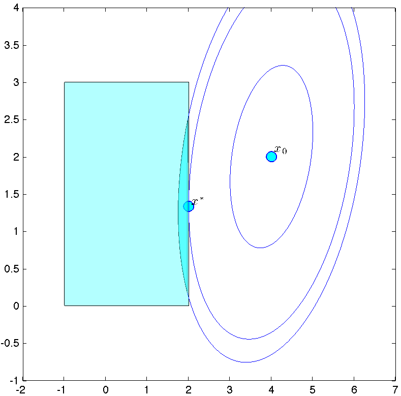Góc nhìn hình học về bài toán tối ưu đồ chơi ở trên. Các đường mức (đường có giá trị không đổi) của hàm mục tiêu được hiển thị. Bài toán tương đương với việc tìm giá trị nhỏ nhất của [latex]t[/latex] sao cho [latex]t=f_0(x)[/latex] với một điểm [latex]x[/latex] khả thi nào đó. Đồ thị cũng cho thấy điểm cực tiểu không ràng buộc của hàm mục tiêu, đặt tại [latex]\hat{x}=(4,2)[/latex]. Một tập [latex]\epsilon[/latex]-dưới tối ưu cho bài toán đồ chơi ở trên được hiển thị (màu đậm hơn), với [latex]\epsilon=0.9[/latex]. Điều này tương ứng với tập hợp các điểm khả thi đạt được giá trị mục tiêu nhỏ hơn hoặc bằng [latex]p^*+\epsilon[/latex].