21 6.2 Formulas with 3-D References
Learning Objectives
- Entering formulas that reference another sheet.
- Using the SUM function to add up multiple sheets.
The Summary sheet in many multiple sheet workbooks is utilized to present totaled information from the other sheets in the file. This is done to give a quick synopsis of all the other sheets in one convenient location. For this reason, the Summary sheet is usually the first sheet in multiple sheet files. Summary sheets “pull” data from the other sheets using three-dimensional (3-D) cell references. In order to distinguish between A3 in the Summary sheet, A3 in the January sheet, A3 in the February sheet, etc.; a 3-D cell reference includes the sheet name along with the cell reference. The syntax to reference a cell in a different sheet is =SheetName!CellRange. So, the cell reference for A15 in the March sheet would be =March!A15.
Let’s start working on our summary sheet by trying out some 3-D formulas:
- Click on the Expenses Summary sheet tab at the bottom of the screen.
- Click on C5 and enter the formula =January!C5. Press Enter.
This will return the amount $700 from cell C5 in the January sheet. - Delete the formula in C5 in the Expenses Summary sheet.
- This time, click on C5 and type =. Then click on the January sheet, and then click on C5.
- Press Enter. This will put the same formula, =January!C5, in cell C5 in the Expenses Summary sheet and will return the value $700. This is the point and click method. This method reduces the potential for making errors, such as misspellings or typing the wrong amount.
- In cell C6 in the Expenses Summary sheet, try entering a formula for the Power amount in the April sheet. You should get $135 as the Power amount, and the formula should be =April!C6.
- Delete the formulas in cells C5 and C6 in the Expenses Summary sheet.
For the Annual Amounts in C5:C13 in the Expenses Summary sheet, we don’t need the amount from a single month’s sheets; instead, we need the sum of all the entries in all the monthly sheets. So, we need to sum three-dimensionally through all twelve month sheets.
Let’s try adding up all the monthly amounts in our Expenses Summary sheet:
- Click in C5 in the Expenses Summary sheet.
- Type =SUM(. (Make sure to type the open parentheses!)
- Click on the January sheet.
- Hold the SHIFT key down and click on the December sheet.
- Click on C5 again and press ENTER. Cell C5 should display the sum amount of $8,400.
- Click on C5 in the Expenses Summary sheet. In the formula bar, you should see the following formula: =SUM(January:December!C5). This formula tells Excel to SUM cell C5 in the sheets January through December.
- Let’s try another 3-D SUM together. Click on C6.
- Type =SUM(. (Make sure to type the open parentheses!)
- Click on the January sheet.
- Hold the SHIFT key down and click on the December sheet.
- Click on C6 again and press ENTER. Cell C6 should now display the sum amount of $1,610.
- Click on C6 in the Expenses Summary sheet. In the formula bar, you should see the following formula: =SUM(January:December!C6).
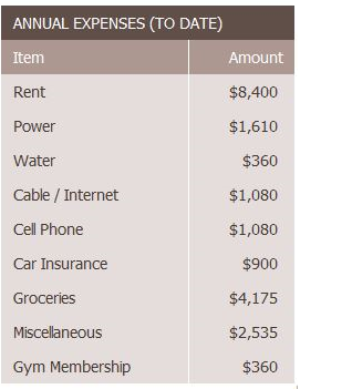
If you feel comfortable with these 3-D formulas, you can copy C6 down through C13 to fill in the rest of the formulas. If you’re not quite comfortable yet, keep practicing the above steps to add 3-D formulas to cells C7:C13. When you’re done, your Expenses Summary sheet should match Figure 6.7.

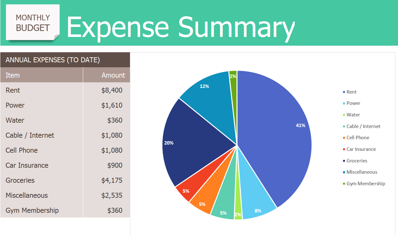
While our 3-D formulas are complete in the Expenses Summary sheet, our summary feels like it is lacking something. Let’s add a visual representation of our summary numbers to the sheet.
- Highlight cells B5:C13 in the Expenses Summary sheet.
- Click on Pie Chart in the Insert tab in the ribbon and select the 2-D pie.
- Move and resize the pie chart so that it fills cells D3:J15.
- Delete the chart title.
- Move the legend to the right side of the chart. Resize the legend as needed.
- Add percentage data labels to the pie slices. Format the data labels to be bold with white font color. Your complete Expenses Summary sheet should look like Figure 6.8 below.
- Check the spelling on all of the worksheets and make any necessary changes.
- Save your file. If you’re printing your assignment at this point, print ONLY the Summary sheet in regular and formula view. Close your file.

Skill Refresher
To SUM across sheets:
- Click on the cell where you want the 3-D SUM to appear.
- Type =SUM(
- Click on the leftmost sheet in the group of sheets you want to sum.
- Hold the SHIFT key down and click on the rightmost sheet in the group of sheets you want to sum.
- Click on the cell in the sheet you’re in that you want to sum.
- Press ENTER.
Skill Refresher
3-D References in Formulas
To reference a cell in another sheet, use the formula syntax =SheetName!CellAddress.
To enter a 3-D reference:
- Click on the cell where you want the formula to appear and type =.
- Click on the sheet with the cell you want.
- Click on the cell in the sheet you want and press ENTER.
Key Takeaways
- 3-D references in formulas allow you to use data from one or more sheets on another sheet.
Attribution
“6.2 Formulas with 3-D References” by Mary Schatz and Diane Shingledecker, Portland Community College is licensed under CC BY 4.0

