2.12: Optimization
2.12: Optimization
We have used derivatives to help find the maximums and minimums of some functions given by equations, but it is very unlikely that someone will simply hand you a function and ask you to find its extreme values. More typically, someone will describe a problem and ask your help in maximizing or minimizing something:
- What is the largest volume package which the post office will take?
- What is the quickest way to get from here to there?
- What is the least expensive way to accomplish some task?
In this section, we’ll discuss how to find these extreme values using calculus.
The second derivative of a function and the extrema of the function
The concavity of a function can also help us determine whether a critical point is a maximum or minimum or neither. For example, if a point is at the bottom of a concave up function, then the point is a minimum.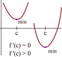
The Second Derivative Test for Extrema
- If [latex]f''(c) \lt 0[/latex] (negative) then [latex]f[/latex] is concave down and has a local maximum at [latex]x = c[/latex].
- If [latex]f''(c) \gt 0[/latex] (positive) then [latex]f[/latex] is concave up and has a local minimum at [latex]x = c[/latex].
- If [latex]f''(c) = 0[/latex] then [latex]f[/latex] may have a local maximum, a minimum or neither at [latex]x = c[/latex].
The cartoon faces can help you remember the Second Derivative Test.

Example 1
[latex]f(x) = 2x^3 - 15x^2 + 24x - 7[/latex] has critical numbers [latex]x =[/latex] 1 and 4. Use the Second Derivative Test for Extremes to determine whether [latex]f(1)[/latex] and [latex]f(4)[/latex] are maximums or minimums or neither.
Answer: We need to find the second derivative:
[latex]\begin{align*} f(x) & = 2x^3 - 15x^2 + 24x - 7\\ f'(x) & = 6x^2 - 30x + 24\\ f''(x) & = 12x - 30 \end{align*}[/latex]
Then we just need to evaluate [latex]f''[/latex] at each critical number:
[latex]x = 1: f''(1)=12(1)-30 \lt 0[/latex], so there is a local maximum at [latex]x = 1[/latex].
[latex]x = 4: f''(4)=12(4)-30 \gt 0[/latex], so there is a local minimum at [latex]x = 4[/latex].
Many students like the Second Derivative Test. The Second Derivative Test is often easier to use than the First Derivative Test. You only have to find the sign of one number for each critical number rather than two. And if your function is a polynomial, its second derivative will probably be a simpler function than the derivative.
However, if you needed a product rule, quotient rule, or chain rule to find the first derivative, finding the second derivative can be a lot of work. Also, even if the second derivative is easy, the Second Derivative Test doesn’t always give an answer. The First Derivative Test will always give you an answer.
Use whichever test you want to. But remember - you have to do some test to be sure that your critical point actually is a local max or min.
Video Demonstration
Finding local extrema:
© 2014 Eric Bancroft
Global Maxima and Minima
Endpoint Extremes
To find Global Extremes...
- If the function is continuous on its domain and has only one critical point, and this point is a local extreme, then the point is also the global extreme.
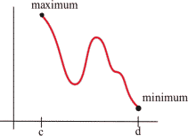
- If there are endpoints, find the global extremes by comparing [latex]y[/latex]-values at all the critical points and at the endpoints.
- When in doubt, graph the function to be sure. (However, unless the problem explicitly tells you otherwise, it is not enough to just use the graph to get your answer.)
Example 2
| [latex] x[/latex] | [latex] f(x)[/latex] |
| [latex]-2[/latex] | [latex]f(-2) = (-2)^3 - 3(-2)^2 - 9(-2) + 5=3[/latex] |
| [latex]-1[/latex] | [latex]f(-1) = (-1)^3 - 3(-1)^2 - 9(-1) + 5=10[/latex] |
| [latex]3[/latex] | [latex]f(3) = (3)^3 - 3(3)^2 - 9(3) + 5=-22[/latex] |
| [latex]6[/latex] | [latex]f(6) = (6)^3 - 3(6)^2 - 9(6) + 5=59[/latex] |
Caution
Video Demonstration
Finding the global extrema of a continuous function on a closed interval
© 2014 Eric Bancroft
If there's only one critical point
If the function that is continuous has only one critical point and the point is a local max (or min), then the point must be the global max (or min). To see this, think about the geometry. Look at the graph on the left - there is a local max, and the graph goes down on either side of the critical point. Suppose there was some other point that was higher - then the graph would have to turn around. But that turning point would have shown up as another critical point. If there’s only one critical point, then the graph can never turn back around.
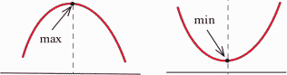
When in doubt, graph it and look.
If you are trying to find a global max or min on an open interval (or the whole real line), and there is more than one critical point, then you need to look at the graph to decide whether there is a global max or min. Be sure that all your critical points show in your graph, and that you graph beyond them - that will tell you what you want to know.
Example 3
Find the global max and min of [latex]f(x) = x^3 - 6x^2 + 9x + 2[/latex].
Answer: First note that this function is a polynomial, so it is continuous on [latex](-\infty,\infty)[/latex].
We have previously found that [latex](1, 6)[/latex] is a local max and [latex](3, 2)[/latex] is a local min. This is not a closed interval, and there are two critical points, so we must turn to the graph of the function to find global max and min.
The graph of [latex]f[/latex] shows that points to the left of [latex]x = 4[/latex] have [latex]y[/latex]-values greater than [latex]6[/latex], so [latex](1, 6)[/latex] is not a global max. Likewise, if [latex]x[/latex] is negative, [latex]y[/latex] is less than [latex]2[/latex], so [latex](3, 2)[/latex] is not a global min. There are no endpoints, so we’ve exhausted all the possibilities. Therefore, this function does not have a global maximum or minimum.

Optimization
The process of finding maxima or minima is called optimization. The function we're optimizing is called the objective function (or objective equation). The objective function can be recognized by its proximity to "est" words (greatest, least, highest, farthest, most). Look at the garden store example; the cost function is the objective function.
In many cases, there are two (or more) variables in the problem. In the garden store example again, the length and width of the enclosure are both unknown. If there is an equation that relates the variables we can solve for one of them in terms of the others, and write the objective function as a function of just one variable. Equations that relate the variables in this way are called constraint equations . The constraint equations are always equations, so they will have equals signs. For the garden store, the fixed area relates the length and width of the enclosure. This will give us our constraint equation.
Optimization Story Problem Technique
- Translate the word statement of the problem line by line into a picture (if that applies) and into math. This is often the hardest step!
- Identify the objective function. Look for words indicating a largest or smallest value.
- If you seem to have two or more variables, find the constraint equation. Think about the meaning of the word constraint, and remember that the constraint equation will have an equals sign.
- Solve the constraint equation for one variable and substitute into the objective function. Now you have an equation of one variable.
- Use calculus to find the optimum values. (Take derivative, find critical points, test. Don't forget to check the endpoints!)
- Look back at the question to make sure you answered what was asked. Translate your number answer back into words.
Video Demonstration
Applied Optimization
© 2014 Eric Bancroft
Example 1
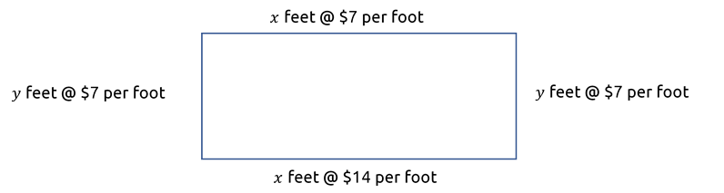
The manager of a garden store wants to build a 600 square foot rectangular enclosure on the store's parking lot in order to display some equipment. Three sides of the enclosure will be built of redwood fencing, at a cost of $7 per running foot. The fourth side will be built of cement blocks, at a cost of $14 per running foot. Find the dimensions of the least costly such enclosure.
Answer: dimensions of enclosure?
Objective: minimize cost
Objective function: [latex]C=14x+7y+7x+7y=21x+14y[/latex]
We must rewrite the objective function as a function of one variable, i.e., eliminate one of the two variables.
Since we have a condition on the area size, we have [latex]A = xy = 600[/latex] where [latex]A[/latex] is the area. Solving for [latex]x[/latex] we get [latex]x=\frac{600}{y}[/latex]. We then substitute the value of [latex]x[/latex] into [latex]C[/latex]:
[latex]C(y)=21\left(\frac{600}{y}\right)+14y=\frac{12600}{y}+14y=12600y^{-1}+14y[/latex]
Now we have a function of just one variable, so we can find the minimum, if it exists, using calculus. For that we need to find the potential locations for the minimum, i.e, we need to identify the critical numbers of [latex]C(y)[/latex].
First, the domain of [latex]C[/latex]:
mathematically: [latex]C(y)=12600y^{-1}+14y[/latex] is defined everywhere except when [latex]y=0[/latex]
contextually: [latex]y[/latex] represents the length of the enclosure, which must be a positive value.
So [latex]y>0[/latex] and the domain is [latex](0,\infty)[/latex], an open interval.
In addition, the objective function is continuous everywhere on its domain.
Then we need to find the critical numbers, which will give us the potential local minima or maxima for the cost. So we need to find out where [latex]C'(y)[/latex] is zero or undefined. Since
[latex]C'(y)=12600(-1)y^{-1-1}+14=-12600y^{-2}+14=-\frac{12600}{y^2}+14[/latex]
we have that [latex]C'(y)[/latex] is undefined for [latex]y = 0[/latex], which is not in the domain and so [latex]y=0[/latex] is not a critical number. We also have that [latex]C' (y)= 0[/latex] when
[latex]\begin{align*} -\frac{12600}{y^2}+14&=0\\\\ \Rightarrow\frac{-12600+14y^2}{y^2}&=0\\\\ \Rightarrow-12600+14y^2&=0\\\\ \Rightarrow y^2&=\frac{12600}{14}=900\\\\ \Rightarrow y&=\pm 30 \end{align*}[/latex]
Since only [latex]y=30[/latex] is in the domain, it is the only critical number. Therefore [latex]y=30[/latex] gives the only potential maximum or minimum cost.
We now use the second derivative test to determine the answer, if possible:
[latex]C''(y)=-12600(-2)y^{-2-1}+0=25200y^{-3}=\frac{25200}{y^3} \Rightarrow C''(30)\gt 0[/latex]
so [latex]y=30[/latex] gives a local minimum.
Since this is the only critical point in the domain, which is an open interval, this must give the global minimum for the cost.
Going back to our constraint function, we can find that when [latex]y = 30[/latex], [latex]x = \frac{600}{30}=20[/latex].
Therefore, the dimensions of the enclosure that minimize the cost are 20 feet by 30 feet, where the more expensive side is 20 feet long.
Video Demonstration
Examples
© 2014 Eric Bancroft
When trying to maximize their revenue, businesses also face the constraint of consumer demand. While a business would love to see lots of products at a very high price, typically demand decreases as the price of goods increases. In simple cases, we can construct that demand curve to allow us to maximize revenue.
Section Exercises
Work on the following exercises. Discuss your solutions with your peers and/or course instructor.
IC4NITS Exercises 2.12 - Optimization
