2.10: Curve Sketching
2.10: Curve Sketching
This section examines some of the interplay between the shape of the graph of [latex]f[/latex] and the behavior of [latex]f'[/latex]. If we have a graph of [latex]f[/latex], we will see what we can conclude about the values of [latex]f'[/latex]. If we know values of [latex]f'[/latex], we will see what we can conclude about the graph of [latex]f[/latex]. We will also utilize the information from [latex]f''[/latex] that we learning in the last section.
Video Demonstration
Curve sketching
© 2014 Eric Bancroft
First Derivative Information
Definitions
The function [latex]f(x)[/latex] is increasing on [latex](a,b)[/latex] if [latex]a \lt x_1 \lt x_2 \lt b[/latex] implies [latex]f( x_1 ) \lt f( x_2 )[/latex].
The function [latex]f(x)[/latex] is decreasing on [latex](a,b)[/latex] if [latex]a \lt x_1 \lt x_2 \lt b[/latex] implies [latex]f( x_1 ) \gt f( x_2 )[/latex].
Graphically, [latex]f[/latex] is increasing (decreasing) if, as we move from left to right along the graph of [latex]f[/latex], the height of the graph increases (decreases).
These same ideas make sense if we consider [latex]h(t)[/latex] to be the height (in feet) of a rocket at time [latex]t[/latex] seconds. We naturally say that the rocket is rising or that its height is increasing if the height [latex]h(t)[/latex] increases over a period of time, as [latex]t[/latex] increases.
Example 1
List the intervals on which the function shown is increasing or decreasing.
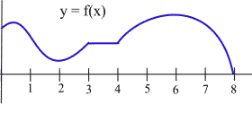
Answer:
[latex]f[/latex] is increasing on the intervals [0,1], [ 2,3] and [4,6].
[latex]f[/latex] is decreasing on [1,2] and [6,8].
On the interval [3,4] the function is not increasing or decreasing – it is constant.
First Derivative Information about Shape
First Shape Theorem (part a)
For a function [latex]f[/latex] which is differentiable on an interval [latex](a,b)[/latex];
- if [latex]f[/latex] is increasing on [latex](a,b)[/latex], then [latex]f'(x) \geq 0[/latex] for all [latex]x[/latex] in [latex](a,b)[/latex].
- if [latex]f[/latex] is decreasing on [latex](a,b)[/latex], then [latex]f'(x) \leq 0[/latex] for all [latex]x[/latex] in [latex](a,b)[/latex].
- if [latex]f[/latex] is constant on [latex](a,b)[/latex], then [latex]f'(x) = 0[/latex] for all [latex]x[/latex] in [latex](a,b)[/latex].
Example 2
The graph shows the height of a helicopter during a period of time. Sketch the graph of the upward velocity of the helicopter, [latex]\frac{dh}{dt}[/latex].
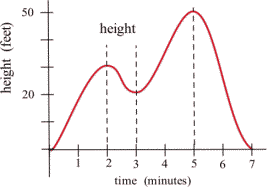
Answer:
Notice that the [latex]h(t)[/latex] has a local maximum when [latex]t = 2[/latex] and [latex]t = 5[/latex], and so [latex]v(2) = 0[/latex] and [latex]v(5) = 0[/latex]. Similarly, [latex]h(t)[/latex] has a local minimum when [latex]t = 3[/latex], so [latex]v(3) = 0[/latex].
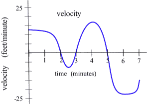
When [latex]h[/latex] is increasing, [latex]v[/latex] is positive. When [latex]h[/latex] is decreasing, [latex]v[/latex] is negative.
Using this information, we can sketch a graph of [latex]v(t) = \frac{dh}{dt}[/latex].
The next theorem is almost the converse of the First Shape Theorem and explains the relationship between the values of the derivative and the graph of a function from a different perspective. It says that if we know something about the values of [latex]f'[/latex], then we can draw some conclusions about the shape of the graph of [latex]f[/latex].
First Shape Theorem (part b)
For a function [latex]f[/latex] which is differentiable on an interval [latex]I[/latex];
- if [latex]f'(x) \gt 0[/latex] for all [latex]x[/latex] in the interval [latex]I[/latex], then [latex]f[/latex] is increasing on [latex]I[/latex].
- if [latex]f'(x) \lt 0[/latex] for all [latex]x[/latex] in the interval [latex]I[/latex], then [latex]f[/latex] is decreasing on [latex]I[/latex].
- if [latex]f'(x) = 0[/latex] for all [latex]x[/latex] in the interval [latex]I[/latex], then [latex]f[/latex] is constant on [latex]I[/latex].
Example 3
Use information about the values of [latex]f'[/latex] to help graph [latex]f(x)=x^3-6x^2+9x+1[/latex].
Answer: graph of [latex]f(x)[/latex]?
First determine the domain: [latex]f[/latex] is a polynomial so the domain is all real numbers.
Then identify the critical numbers:
[latex]f'(x) = 3x^2 - 12x + 9 = 3(x - 1)(x - 3)[/latex]
[latex]f'[/latex] is a polynomial so it is always defined.
[latex]f'(x) = 0[/latex] only when [latex]x = 1[/latex] or [latex]x = 3[/latex], both of which are in the domain of [latex]f[/latex]
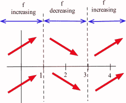
Therefore, the critical numbers for [latex]f[/latex] are [latex]x = 1[/latex] and [latex]x = 3[/latex], and they divide the domain into three intervals: [latex](-\infty, 1)[/latex], [latex](1,3)[/latex], and [latex](3, \infty)[/latex].
On each of these intervals, the function is either always increasing or always decreasing.
If [latex]x \lt 1[/latex], then [latex]f '(x) =[/latex] 3(negative number)(negative number) [latex]\gt 0[/latex] so [latex]f[/latex] is increasing.
If [latex]1 \lt x \lt 3[/latex], then [latex]f'(x) =[/latex] 3(positive number)(negative number) [latex]\lt 0[/latex] so f is decreasing.
If [latex]x \gt 3[/latex], then [latex]f'(x) =[/latex] 3(positive number)(positive number) [latex]\gt 0[/latex] so [latex]f[/latex] is increasing.
Even though we don't know the value of [latex]f[/latex] anywhere yet, we do know a lot about the shape of the graph of [latex]f[/latex]: as we move from left to right along the [latex]x[/latex]-axis, the graph of [latex]f[/latex] increases until [latex]x = 1[/latex], then the graph decreases until [latex]x = 3[/latex], and then the graph increases again. The graph of [latex]f[/latex] makes "turns" when [latex]x = 1[/latex] and [latex]x = 3[/latex]; it has a local maximum at [latex]x = 1[/latex], and a local minimum at [latex]x = 3[/latex].
To plot the graph of [latex]f[/latex], we still need to evaluate [latex]f[/latex] at a few values of [latex]x[/latex], but only at a very few values. [latex]f(1) = 5[/latex], and (1,5) is a local maximum of [latex]f[/latex]. [latex]f(3) = 1[/latex], and (3,1) is a local minimum of [latex]f[/latex]. The resulting graph of [latex]f[/latex] is shown here.
Second Derivative Information
Until now, we've only used first derivative information, but we could also use information from the second derivative to provide more information about the shape of the function.
Second Derivative Information about Shape
- If [latex]f[/latex] is concave up on [latex](a,b)[/latex], then [latex]f''(x) \geq 0[/latex] for all [latex]x[/latex] in [latex](a,b)[/latex].
- If [latex]f[/latex] is concave down on [latex](a,b)[/latex], then [latex]f''(x) \leq 0[/latex] for all [latex]x[/latex] in [latex](a,b)[/latex].
The converse of both of these are also true:
- If [latex]f''(x) \geq 0[/latex] for all [latex]x[/latex] in [latex](a,b),[/latex] then [latex]f[/latex] is concave up on [latex](a,b)[/latex].
- If [latex]f''(x) \leq 0[/latex] for all [latex]x[/latex] in [latex](a,b),[/latex] then [latex]f[/latex] is concave down on [latex](a,b)[/latex].
Video Demonstration
Curve sketching: Example A
© 2014 Eric Bancroft
Example 4
Use information about the values of [latex]f''[/latex] to help determine the intervals on which the function [latex]f(x) = x^3 - 6x^2 + 9x + 1[/latex] is concave up and concave down.
Answer: concavity intervals?
First, the domain. The function is a polynomial so its domain is all real numbers.
A function is concave up when its second derivative is positive and the function is concave down when its second derivative is negative. Therefore, to determine concavity, we need the second derivative:
[latex]f'(x)=3x^2-12x+9[/latex], so [latex]f''(x)=6x-12[/latex]
The concavity will change at inflection points, so we need to identify them, i.e., we need to identify for which [latex]x[/latex] in the domain is [latex]f''(x)[/latex] undefined or equal to zero.
Since [latex]f''[/latex] is a polynomial, it is never undefined.
For [latex]f''(x)=0[/latex] we have that [latex]6x-12=0[/latex], and so [latex]x = 2[/latex], which is in the domain of [latex]f[/latex].
Therefore, the only potential inflection point will occur at [latex]x=2[/latex].
We now split the domain into subintervals using the potential inflection points and we investigate the sign of [latex]f''[/latex] on each subinterval to determine the concavity of [latex]f[/latex]: [latex](-\infty,2)[/latex] and [latex](2,\infty)[/latex].
For [latex]x \lt 2[/latex], the second derivative is negative (for example, [latex]f''(0)=6(0)-12=-12[/latex]), so [latex]f[/latex] is concave down on [latex](-\infty, 2)[/latex].
For [latex]x \gt 2[/latex], the second derivative is positive (test [latex]f''[/latex] on, say, [latex]x=4[/latex]), so [latex]f[/latex] is concave up on [latex](2,\infty)[/latex].
We could have incorporated this concavity information when sketching the graph for the previous example, and indeed we can see the concavity reflected in the graph using a graphing calculator: link to graph.
Video Demonstration
Curve sketching: Example B
© 2014 Eric Bancroft
Example 5
Use information about the values of [latex]f'[/latex] and [latex]f''[/latex] to help graph [latex]f(x)=x^{2/3}[/latex].
Answer: graph of [latex]f[/latex]?
Domain of [latex]f[/latex] is all real numbers (odd root function).
Critical numbers?
[latex]f'(x)=\frac{2}{3}x^{-1/3}[/latex]
[latex]f'(x)[/latex] is undefined at [latex]x = 0[/latex], which is also in the domain.
[latex]f'(x)[/latex] is never zero.
Therefore the only critical number of [latex]f[/latex] is [latex]x=0[/latex]
Potential inflection points?
[latex]f''(x)=-\frac{2}{9}x^{-4/3}[/latex]
[latex]f''(x)[/latex] is also undefined at [latex]x = 0[/latex], which is in the domain.
[latex]f''(x)[/latex] is also never zero.
Therefore there is a potential inflection point at [latex]x=0[/latex].
This gives us only one point of interest, which we use to subdivide the domain into subintervals: [latex]x \lt 0[/latex] and [latex]x \gt 0[/latex].
On the interval [latex]x \lt 0[/latex], we could test out a value like [latex]x = -1[/latex]:
[latex]f'(-1)=\frac{2}{3}(-1)^{-1/3}=-\frac{2}{3}[/latex]
[latex]f''(-1)=-\frac{2}{9}(-1)^{-4/3}=-\frac{2}{9}[/latex]
Since [latex]f'(x)[/latex] is negative and [latex]f''(x)[/latex] is negative, we can conclude that the function is decreasing and concave down on this interval.
On the interval [latex]x \gt 0[/latex], we could test out a value like [latex]x = 1[/latex]:
[latex]f'(1)=\frac{2}{3}(1)^{-1/3}=\frac{2}{3}[/latex]
[latex]f''(1)=-\frac{2}{9}(1)^{-4/3}=-\frac{2}{9}.[/latex]
Since [latex]f'(x)[/latex] is positive and [latex]f''(x)[/latex] is negative, we can conclude that the function is increasing and concave down on this interval.
We can also calculate that [latex]f(0)=0[/latex], giving us a base point for the graph. Using this information, we can conclude the graph must look like this:

Video Demonstration
Curve sketching: Example C
© 2014 Eric Bancroft
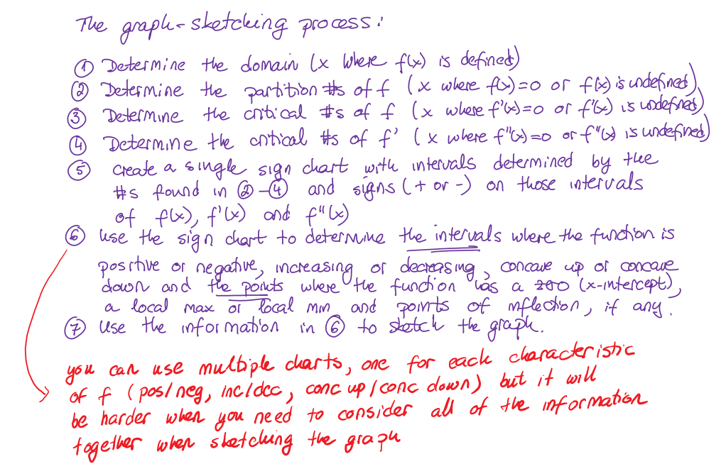
One can summarize the curve-sketching process as follows:
Example 6
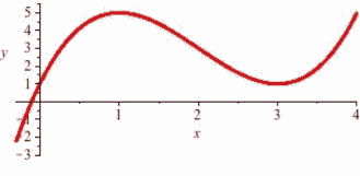
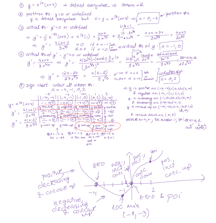
Use the first and the second derivative to sketch the graph of the following function:
[latex]f(x)=x^{1/3}(x+4)[/latex]
Answer: graph of [latex]f[/latex]?
Sketching without an Equation
Of course, graphing calculators and computers are great at graphing functions. Calculus provides a way to illuminate what may be hidden or out of view when we graph using technology. More importantly, calculus gives us a way to look at the derivatives of functions for which there is no equation given. We already saw the idea of this back in Section 2.3 where we sketched the derivative of two graphs by estimating slopes on the curves.
We can summarize all the derivative information about shape in a table.
Summary of Derivative Information about the Graph
| [latex]f(x)[/latex] | Increasing | Decreasing | Concave Up | Concave Down |
| [latex]f'(x)[/latex] | [latex]+[/latex] | [latex]-[/latex] | Increasing | Decreasing |
| [latex]f''(x)[/latex] | [latex]+[/latex] | [latex]-[/latex] |
When [latex]f'(x) = 0[/latex], the graph of [latex]f[/latex] may have a local max or min.
When [latex]f''(x) = 0[/latex], the graph of [latex]f[/latex] may have an inflection point.
Section Exercises
Work on the following exercises. Discuss your solutions with your peers and/or course instructor.
IC4NITS Exercises 2.10 - Curve Sketching
