2.1 Limits and Continuity
2.1 Limits and Continuity
As we saw in the previous chapter, not every algebraic or transcendental function is defined on all real numbers. The domain of a function will sometimes be restricted due to the algebraic operations such as division and (even) roots or due to other types of restrictions. To fully understand the behaviour of the relationship represented through such functions, we would also need to understand the behaviour of the function in the immediate neighbourhood of values that are just outside of the domain.
Additionally, sometimes there are values in the domain where there are sudden, perhaps unexpected, changes to the output, indicating a special behavioural characteristic of the relationship we are studying.
Sometimes things are nice and smooth, even if "bumpy" over a period, and this is also a valuable characteristic to identify, a characteristic we call continuity. For some functions, the characteristic of "smoothness", or continuity, is maintained throughout the relationship, such as in the case of a linear, quadratic or a general polynomial function. Establishing when the continuity characteristic is present is really important. It will allow us to make many inferences and use a variety of mathematical tools that will help us understand the relationship represented through the given function even better.
Even understanding the "bumpiness" of a smooth, continuous function is important in order to understand the behaviour of the relationship represented by the function. How fast are the results, the output values of the function, growing or falling as we increase or decrease the input values? Where are the tops of the hills and bottoms of the valleys, i.e., the highest or the lowest results? Those questions can only be answered by understanding the change in the output in the immediate neighbourhood of each of the points along the relationship.
You will also recall from our summaries of general characteristics of the basic types of functions that the functions behave in a specific way as we take our inputs to the extreme ends of the real numbers, towards positive or negative infinity. Sometimes they exhibit perpetual growth and sometimes decay, or are bound above or below by an imaginary ceiling or floor, a so-called horizontal asymptote. These characteristics are important to understand when we are considering a model of some real-life problem and we ask the (natural) question: what would happen to my result if I keep on increasing (or decreasing) such-and-such, whatever the input value happens to represent.
To get answers to all of these questions, we would first need to identify the places where our function "breaks" or "falls" or "jumps", and we'd need a tool to measure in some way our results at the extremes we're not able to reach. For all of that, we need the mathematical concept of a limit of a function.
 |
 |
Limit of a function
The word that underpins all of the questions discussed above is that of "approach". If the input value is approaching a particular value, say [latex]a[/latex], does the value of the function, or the output, approach some specific value, say [latex]L[/latex]? If yes, we call that value [latex]L[/latex] the limit of the function. The mathematical concept of a limit gives us better language with which to discuss the idea of “approaches.”
Definition of limit of a function
Formal definition:
The function [latex]f(x)[/latex] has a limit [latex]L[/latex] as [latex]x[/latex] approaches [latex]a[/latex] if and only if for every [latex]\epsilon\gt 0[/latex] there exists a [latex]\delta\gt 0[/latex] such that for every [latex]x[/latex] that satisfies [latex]|x-a|\lt\delta[/latex] we have that [latex]|f(x)-L|\lt \epsilon[/latex]
Conceptual definition:
If the values of [latex]f(x)[/latex] get closer and closer, as close as we want, to one number [latex]L[/latex] as we take values of [latex]x[/latex] very close to (but not equal to) a number [latex]a[/latex], then we say " the limit of [latex]f(x)[/latex] as [latex]x[/latex] approaches [latex]a[/latex] is [latex]L[/latex] " and we write [latex]\lim\limits_{x\to a} f(x)=L.[/latex]
The conceptual definition will be sufficient for our purposes in this course.
In either case, we use very specific mathematical notation to denote the limit of a function:
If the function [latex]f(x)[/latex] has a limit value [latex]L[/latex] as the input variable [latex]x[/latex] approaches some value [latex]a[/latex], we write
[latex]\lim\limits_{x\to a} f(x)=L[/latex]
and we read this as "the limit of [latex]f[/latex] of [latex]x[/latex] as [latex]x[/latex] approaches [latex]a[/latex] is [latex]L[/latex]."
We can also write
[latex]f(x)\to L[/latex] as [latex]x\to a[/latex]
The symbol "[latex]\to[/latex]" means "approaches" or, less formally, "gets very close to" so we read this as "[latex]f[/latex] of [latex]x[/latex] approaches [latex]L[/latex] as [latex]x[/latex] approaches [latex]a[/latex]."
Note:
- [latex]f(a)[/latex] is a single number that describes the behavior (value) of [latex]f(x)[/latex] at the input value [latex]x = a[/latex].
- [latex]\lim\limits_{x\to a} f(x)[/latex] is a single number that describes the behavior of [latex]f(x)[/latex] near, but NOT at , the input value [latex]x = a[/latex].
Example 1
Use the graph of [latex]y = f(x)[/latex] in the figure below to determine the following limits:
- [latex]\lim\limits_{x\to 1} f(x)[/latex]
- [latex]\lim\limits_{x\to 2} f(x)[/latex]
- [latex]\lim\limits_{x\to 3} f(x)[/latex]
- [latex]\lim\limits_{x\to 4} f(x)[/latex]
1. As [latex]x[/latex] approaches [latex]1[/latex] from either side, the values of [latex]f(x)[/latex] are approaching [latex]y = 2[/latex]. Therefore,
[latex]\lim\limits_{x\to 1}f(x)=2[/latex]
Note that, in this example, it so happens that [latex]f(1) = 2[/latex], but that is irrelevant for the limit. The only thing that matters is what happens for [latex]x[/latex] close to [latex]1[/latex] but [latex]x \neq 1[/latex].
2. We can see that [latex]f(2)[/latex] is undefined, but we only care about the behavior of [latex]f(x)[/latex] for [latex]x[/latex] close to 2 but not equal to 2. When [latex]x[/latex] approaches [latex]2[/latex] from either side, the values of [latex]f(x)[/latex] approach [latex]3[/latex], and so
[latex]\lim\limits_{x\to 2}f(x)=3[/latex]
3. When [latex]x[/latex] is approaching [latex]3[/latex] either from the left or from the right, the values of [latex]f(x)[/latex] are approaching [latex]1[/latex], so
[latex]\lim\limits_{x\to 3}f(x)=1[/latex]
Note that for this limit it is completely irrelevant that [latex]f(3) = 2[/latex], We only care about what happens to [latex]f(x)[/latex] for [latex]x[/latex] close to and not equal to [latex]3[/latex].
4. This one is harder and we need to be careful. When [latex]x[/latex] is approaching [latex]4[/latex] from the left side, i.e., it is close and slightly less than 4, then the values of [latex]f(x)[/latex] are approaching [latex]2[/latex]. But if [latex]x[/latex] is approaching [latex]4[/latex] from the right side, i.e., it is close and slightly larger than 4, then the values of [latex]f(x)[/latex] are approaching [latex]3[/latex]. Thus, if we only know that [latex]x[/latex] is very close to 4, then we cannot say whether [latex]y = f(x)[/latex] will be close to [latex]2[/latex] or close to [latex]3[/latex] - the answer to that depends on whether [latex]x[/latex] is on the right or the left side of 4. In this situation, if we are in the immediate neighbourhood of [latex]x=4[/latex], [latex]f(x)[/latex] values are not close to a single number, and so we say [latex]f(x)[/latex] does not exist or that [latex]f(x)[/latex] does not have a limit at [latex]4[/latex].
Note that, in this case, it is irrelevant that [latex]f(4) = 1[/latex]. The limit of [latex]f(x)[/latex], as [latex]x[/latex] approaches [latex]4[/latex], would still be undefined if [latex]f(4)[/latex] was [latex]3[/latex] or [latex]2[/latex] or anything else because the limit is all about the value of the function in the neighbourhood of [latex]4[/latex] and not about the value of the function at [latex]4[/latex].
We can also explore limits using tables and using algebra: view video example.
(by Eric Bancroft, licensed under a Creative Commons Attribution-NonCommercial-NoDerivatives 4.0 International License)
Evaluating limits
In the above example we were given a graphical representation of a function and were able to make conclusions about the limit values of the given function by observing its behaviour visually. However, most of the time this is either not possible or feasible or accurate. In particular, if we know the rule (formula) for a function, but do not have its behaviour explicitly visualized through a graph, we have to analyze the rule, using our knowledge of the algebraic operations and, if present, transcendental components involved. Even using graph vizualization tools will not be helpful in most cases, especially if we are seeking precision - we will have to engage in mathematical analysis of the rule that describes the function.
For example, consider the vizualization of the graph of [latex]f(x)=\frac{37\left(4x^{2}-3x-22\right)}{148x^{2}-579x+473}[/latex] using the graphing tool Desmos: link to graph. You can zoom in and out to your heart's content, but you will not be able to discern that, firstly, there is a vertical asymptote at [latex]x=43/37[/latex] and that, secondly, there is a hole in the graph at [latex]x=11/4[/latex]. To get that information you have to analyze the algebra in the formula for the function.
In order to perform such analysis and be able to evaluate the limits, if they exist, we use the following theorem that lays out fundamental properties of limits:
Algebraic Limit Theorem
If [latex]f[/latex] and [latex]g[/latex] are real-valued functions and if [latex]\lim\limits_{x\to a} f(x)[/latex] and [latex]\lim\limits_{x\to a} g(x)[/latex] both exist, then
[latex]\lim\limits_{x\to a} (f+g)(x)=\lim\limits_{x\to a} f(x)+\lim\limits_{x\to a} g(x)[/latex]
[latex]\lim\limits_{x\to a} (f-g)(x)=\lim\limits_{x\to a} f(x)-\lim\limits_{x\to a} g(x)[/latex]
[latex]\lim\limits_{x\to a} (f\cdot g)(x)=\left(\lim\limits_{x\to a} f(x)\right)\cdot\left(\lim\limits_{x\to a} g(x)\right)[/latex]
[latex]\lim\limits_{x\to a} \left(\frac{f}{g}\right)(x)=\dfrac{\lim\limits_{x\to a} f(x)}{\lim\limits_{x\to a} g(x)}[/latex] if [latex]\lim\limits_{x\to a} g(x)\neq 0[/latex]
[latex]\lim\limits_{x\to a} (f(x))^n=\left(\lim\limits_{x\to a} f(x)\right)^n[/latex]
In particular,
[latex]\lim\limits_{x\to a} c=c[/latex]
[latex]\lim\limits_{x\to a} x=a[/latex]
[latex]\lim\limits_{x\to a} x^n=a^n[/latex]
[latex]\lim\limits_{x\to a} \sqrt[n]{x}=\sqrt[n]{a}[/latex]
Example 2
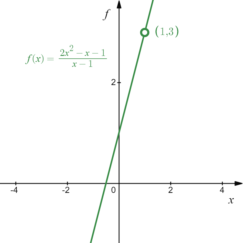
Find [latex]\lim\limits_{x\to 1} \dfrac{2x^2-x-1}{x-1}[/latex].
Answer: [latex]\lim\limits_{x\to 1} \dfrac{2x^2-x-1}{x-1} =?[/latex]
You might note that when [latex]x = 1[/latex], [latex]f(x)[/latex] is not defined. However, remember that this is of no consequence when determining the limit at [latex]x=1[/latex] because with limits we are not interested what happens at that input value - we are only interested in what happens to the function around that value.
To get a sense of what the limit might be, we can sometimes test out the values of the function close to the input value where we are evaluating the limit. For this function we can do it as in the following table but remember that, on top of it being inefficient when unnecessary, it is also not full-proof because you don't ever know if you picked close enough values to be able to make your conclusion.
Here is what the testing out would look like in this example, by trying some "test" values for [latex]x[/latex] which get closer and closer to [latex]1[/latex] from both the left and the right:
| From the left (values slightly less than 1) | From the right (values slightly more than 1) | |||
| [latex]x[/latex] | [latex]f(x)[/latex] | [latex]x[/latex] | [latex]f(x)[/latex] | |
| 0.9 | 2.82 | 1.1 | 3.2 | |
| 0.9998 | 2.9996 | 1.003 | 3.006 | |
| 0.999994 | 2.999988 | 1.0001 | 3.0002 | |
| 0.9999999 | 2.9999998 | 1.000007 | 3.000014 | |
| [latex] \to 1[/latex] | [latex] \to 3[/latex] | [latex] \to 1[/latex] | [latex] \to 3[/latex] | |
The testing seems to indicate that the value of [latex]f(x)[/latex] approaches [latex]3[/latex] as we approach [latex]x=1[/latex] from left and the right, so it appears that the limit of [latex]f(x)[/latex] as [latex]x[/latex] approaches [latex]1[/latex] is [latex]3[/latex]. However, we can't be sure because maybe, just maybe, the function starts to behave differently if we get even closer to [latex]1[/latex]. In addition, the testing is very time and energy consuming and should be reserved for when we have no other options and we, hopefully, have automated ways available for the calculation, such as through writing a programming code to execute the calculations on our behalf.
Instead, let's use the precision of algebra and the properties of limits described in the Algebraic Limit Theorem. We do this by first factoring the original function fully, meaning we write it, to the greatest extend possible, as a product or a quotient of products of simplest terms. For this we will often need to use the method of factoring out a common factor or the quadratic formula:
| [latex]\begin{align*} \lim\limits_{x\to 1}\dfrac{2x^2-x-1}{x-1}&=\dfrac{2(x-1)\left(x+\frac{1}{2}\right)}{x-1}\\ &=\lim\limits_{x\to 1}2\left(x+\frac{1}{2}\right)\\ &=\lim\limits_{x\to 1}2\cdot \left(\lim\limits_{x\to 1}x+\lim\limits_{x\to 1}\frac{1}{2}\right)\\ &=2\left(1+\frac{1}{2}\right)=3 \end{align*}[/latex]Alternatively,[latex]\begin{align*} \lim\limits_{x\to 1}\dfrac{2x^2-x-1}{x-1}&=\dfrac{2(x-1)\left(x+\frac{1}{2}\right)}{x-1}\\\\ &=\lim\limits_{x\to 1}\overbrace{2\left(x+\frac{1}{2}\right)}^{\to 2\left(1+\frac{1}{2}\right)}\\ &=3 \end{align*}[/latex] | Side work: [latex]\rightarrow\\ \leftarrow[/latex] |
Factoring the numerator
[latex]\begin{align*}2x^2-x-1&=a(x-x_1)(x-x_2)\\ &=2(x-1)(x+\frac{1}{2})\end{align*}[/latex] where [latex]\begin{align*} x_{1,2}&=\frac{-b\pm\sqrt{b^2-4ac}}{2a}\\ &=\frac{-(-1)\pm\sqrt{(-1)^2-4\cdot 2\cdot (-1)}}{2\cdot 2}\\ &=\frac{1\pm 3}{4}\\ &=1, -\frac{1}{2} \end{align*}[/latex] |
Example 3
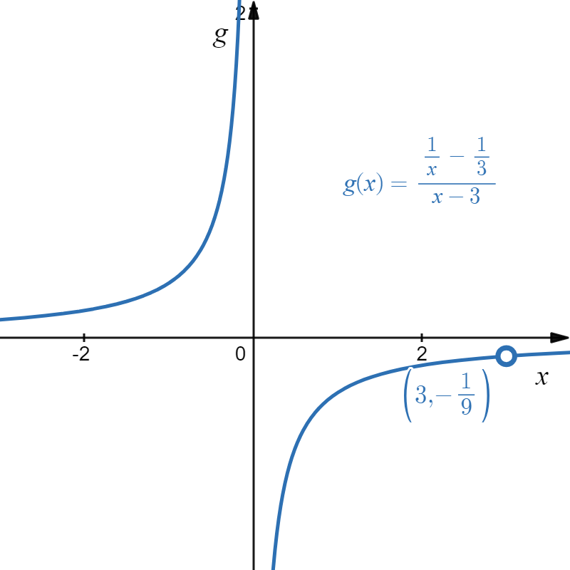
Find [latex]\lim \limits_{x\to 3} \dfrac{\frac{1}{x} -\frac{1}{3} }{x-3}[/latex]
Answer: [latex]\lim \limits_{x\to 3} \dfrac{\frac{1}{x} -\frac{1}{3} }{x-3}=?[/latex]
(General process: analyze, then either evaluate or rewrite (then back to analyze) or break into subcases (then back to analyze))
[latex]\begin{align*} \lim \limits_{x\to 3} \dfrac{\frac{1}{x} -\frac{1}{3} }{x-3}&\overset{rewrite}{=}\lim \limits_{x\to 3} \dfrac{\frac{3-x}{3x}}{x-3}\overset{rewrite}{=}\lim \limits_{x\to 3} \dfrac{3-x}{3x}\cdot \dfrac{1}{x-3}\underset{analyze}{\overset{rewrite}{=}}\lim \limits_{x\to 3} \dfrac{\overbrace{-1}^{\to -1}}{\underbrace{3x}_{\to 9}}\overset{evaluate}{=}-\dfrac{1}{9} \end{align*}[/latex]
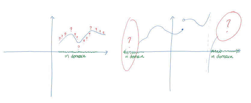
In the last two examples, the function was not defined at the value where we were evaluating the limit yet the function had a limit. In other words, even though the function was not defined for some value [latex]a[/latex], the function behaved "nicely" around [latex]a[/latex], i.e., the value of the function was closer and closer to some specific value, the limit value [latex]L[/latex], in the immediate neighbourhood of [latex]a[/latex]. This kind of behaviour tells us that the function has a hole at [latex]a[/latex]. More formally:
A function [latex]f(x)[/latex] has a hole at [latex](a, L)[/latex] if [latex]f(a)[/latex] is not defined but [latex]\lim \limits_{x\to a}f(x)=L[/latex] for some real value [latex]L[/latex].
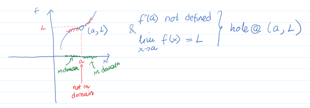
Using the last two examples, we can see that the function defined by [latex]f(x)=\dfrac{2x^2-x-1}{x-1}[/latex] has a hole at [latex](1,3)[/latex] and the function defined by [latex]g(x)=\dfrac{\frac{1}{x} -\frac{1}{3} }{x-3}[/latex] has a hole at [latex]\left(3,-\frac{1}{9}\right)[/latex]. This can be visualized as follows:
 |
 |
View video of another example.
(by Eric Bancroft, licensed under a Creative Commons Attribution-NonCommercial-NoDerivatives 4.0 International License)
One-sided Limits
The left limit of [latex]f(x)[/latex] as [latex]x[/latex] approaches [latex]a[/latex] is [latex]L[/latex] if the values of [latex]f(x)[/latex] get as close to [latex]L[/latex] as we want when [latex]x[/latex] is very close to and left of [latex]a[/latex] (i.e., [latex]x \lt a[/latex]). We write
[latex]\lim\limits_{x\to a^-} f(x)=L[/latex]
The right limit of [latex]f(x)[/latex] as [latex]x[/latex] approaches [latex]a[/latex] is [latex]L[/latex] if the values of [latex]f(x)[/latex] get as close to [latex]L[/latex] as we want when [latex]x[/latex] is very close to and right of [latex]a[/latex] (i.e., [latex]x \gt a[/latex]). We write
[latex]\lim\limits_{x\to a^+} f(x)=L[/latex]
Example 4
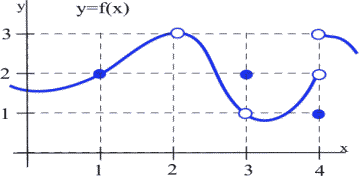
Evaluate the one sided limits of the function [latex]f(x)[/latex] graphed below at [latex]x = 0[/latex] and [latex]x = 1[/latex].

Answer:
As [latex]x[/latex] approaches 0 from the left, the value of the function is getting closer to 1, so [latex]\lim\limits_{x\to 0^-} f(x) = 1.[/latex]
As [latex]x[/latex] approaches 0 from the right, the value of the function is getting closer to 2, so [latex]\lim\limits_{x\to 0^+} f(x) = 2.[/latex]
Note that, since the limit from the left and limit from the right are different, the general limit, [latex]\lim\limits_{x\to 0} f(x)[/latex], does not exist.
At [latex]x[/latex] approaches 1 from either direction, the value of the function is approaching 1, so
[latex]\lim\limits_{x\to 1^-} f(x) = \lim\limits_{x\to 1^+} f(x) = \lim\limits_{x\to 1} f(x) = 1[/latex]
See the analysis of limits through a video of another example.
(by Eric Bancroft, licensed under a Creative Commons Attribution-NonCommercial-NoDerivatives 4.0 International License)
Infinite limits
In some cases where the limit of a function does not exist there may still be valuable information about the behaviour of the function in that specific neighbourhood. One of those cases is when the value of the function either increases or decreases indefinitely to an arbitrarily large positive or negative number, i.e., towards positive or negative infinity. More formally:
Let [latex]f(x)[/latex] be a function defined on both sides of [latex]a[/latex], except possibly at [latex]a[/latex] itself. Then:
- [latex]\lim\limits_{x\to a}f(x)=\infty[/latex] if the value of [latex]f(x)[/latex] can be an arbitrarily large positive number for values of [latex]x[/latex] sufficiently close to [latex]a[/latex]
- [latex]\lim\limits_{x\to a}f(x)=-\infty[/latex] if the value of [latex]f(x)[/latex] can be an arbitrarily large negative number for values of [latex]x[/latex] sufficiently close to [latex]a[/latex]
If the function [latex]f(x)[/latex] approaches positive or negative infinity from either side of some input value [latex]a[/latex], we say that the function has a vertical asymptote at [latex]a[/latex].
Example 5
Evaluate the following and interpret your result:
[latex]\lim\limits_{x\to 2} \dfrac{x-4}{x-2}[/latex]
Answer: [latex]\lim\limits_{x\to 2} \dfrac{x-4}{x-2} =?[/latex]
[latex]\lim\limits_{x\to 2} \dfrac{\overbrace{x-4}^{\to -2}}{\underbrace{x-2}_{\to 0}} =\dfrac{\text{negative number}}{\text{infinitely small number, but is it negative or positive?}}=\text{cannot answer}[/latex]
Split into cases: evaluate while approaching [latex]0[/latex] from the positive side and evaluate while approaching [latex]0[/latex] from the negative side
[latex]\lim\limits_{x\to 2^+} \dfrac{\overbrace{x-4}^{\to -2}}{\underbrace{x-2}_{\to 0^+}} =\dfrac{\text{negative number}}{\text{infinitely small negative number}}=\infty[/latex]
[latex]\lim\limits_{x\to 2^-} \dfrac{\overbrace{x-4}^{\to -2}}{\underbrace{x-2}_{\to 0^+}} =\dfrac{\text{negative number}}{\text{infinitely small positive number}}=-\infty[/latex]
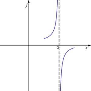
From this, we can conclude that the function [latex]f(x)=\dfrac{x-4}{x-2}[/latex] has a vertical asymptote at [latex]x=2[/latex], with the function approaching [latex]\infty[/latex] from the left and approaching [latex]-\infty[/latex] from the right. We can sketch this as:
Limits at infinities
Up until now we only looked at the behaviour of a function around a specific input value. However, as discussed at the beginning of this section, we are also interested in the long-run behaviour of the function, i.e., we are interested in what happens to the values of the function as we increase or decrease the input values indefinitely. In other words, what happens to the function when the input values approach positive or negative infinity?
More formally:
Let [latex]f(x)[/latex] be a function defined on some interval [latex](a, \infty)[/latex]. Then
[latex]\lim\limits_{x\to\infty}f(x)=L[/latex]
means that the values of [latex]f(x)[/latex] can be made arbitrarily close to [latex]L[/latex] by requiring [latex]x[/latex] to be a sufficiently large positive number. We say that [latex]f(x)[/latex] has a horizontal asymptote at [latex]L[/latex] as [latex]x[/latex] approaches [latex]\infty[/latex].
Similarly, if a function is defined on some interval [latex](-\infty,a)[/latex], then
[latex]\lim\limits_{x\to -\infty}f(x)=L[/latex]
means that the values of [latex]f(x)[/latex] can be made arbitrarily close to [latex]L[/latex] by requiring [latex]x[/latex] to be a sufficiently large negative number. We say that [latex]f(x)[/latex] has a horizontal asymptote at [latex]L[/latex] as [latex]x[/latex] approaches [latex]-\infty[/latex].
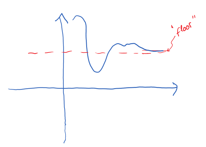
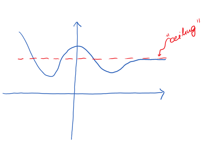
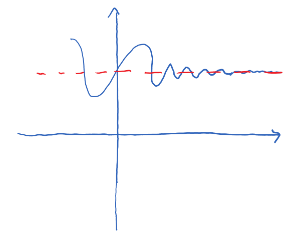
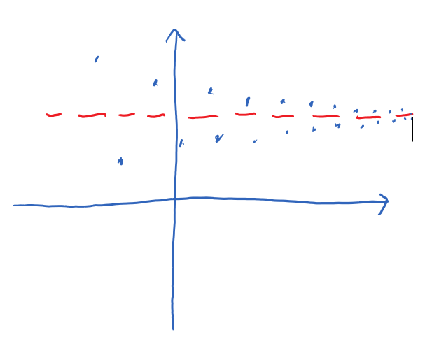
Note that, graphically, a horizontal asymptote means that the values of the function approach a particular value as input increases indefinitely (or decreases indefinitely), but we don't know if the values of the function are decreasing to that value (so the asymptote can be seen as a "floor") or increasing to that value (and asymptote acting as a "ceiling") or are perhaps fluctuating up and down. To determine the behaviour to that level of detail, we would need more investigation and, for that, the calculus tools we'll be discussing in the rest of this chapter will prove helpful. Here are some visual examples of different behaviours around the horizontal asymptote:
 |
 |
 |
 |
Example 6
Determine the following limits and interpret your results:
1. [latex]\lim\limits_{\to\infty}\frac{3x^2-5x}{7x^2+4x-1}[/latex]
2. [latex]\lim\limits_{\to-\infty}\frac{3x^3-5}{7x^2+4x}[/latex]
3. [latex]\lim\limits_{\to\infty}\frac{3x^2-5x}{7x^4-1}[/latex]
Answer:
1. [latex]\lim\limits_{\to\infty}\frac{3x^2-5x}{7x^2+4x-1}=?[/latex] meaning?
[latex]\begin{align*} \lim\limits_{\to\infty}\frac{3x^2-5x}{7x^2+4x-1}&\overset{rewrite}{=}\lim\limits_{\to\infty}\frac{\frac{3x^2}{x^2}-\frac{5x}{x^2}}{\frac{7x^2}{x^2}+\frac{4x}{x^2}-\frac{1}{x^2}}\underset{analyze}{\overset{rewrite}{=}}\lim\limits_{\to\infty}\frac{\overbrace{3-\frac{5}{x}}^{\to 3-0}}{\underbrace{7+\frac{4}{x}-\frac{1}{x^2}}_{\to 7+0-0}}\overset{evaluate}{=}\dfrac{3}{7} \end{align*}[/latex]
Therefore, the function [latex]y=\frac{3x^2-5x}{7x^2+4x-1}[/latex] has a horizontal asymptote at [latex]\dfrac{3}{7}[/latex] as [latex]x\to\infty[/latex].
2. [latex]\lim\limits_{\to -\infty}\frac{3x^3-5}{7x^2+4x}=?[/latex] meaning?
[latex]\begin{align*} \lim\limits_{\to -\infty}\frac{3x^3-5}{7x^2+4x}&\overset{rewrite}{=}\lim\limits_{\to\infty}\frac{\frac{3x^3}{x^2}-\frac{5}{x^2}}{\frac{7x^2}{x^2}+\frac{4x}{x^2}}\underset{analyze}{\overset{rewrite}{=}}\lim\limits_{\to -\infty}\frac{\overbrace{3x-\frac{5}{x}}^{\to -\infty}}{\underbrace{7+\frac{4}{x}}_{\to 7+0-0}}\overset{evaluate}{=}-\infty \end{align*}[/latex]
Therefore, the function [latex]y=\frac{3x^3-5}{7x^2+4x}[/latex] does not have a horizontal asymptote as [latex]x\to -\infty[/latex] and, in fact, decreases infinitely to arbitrarily large negative numbers.
3. [latex]\lim\limits_{\to\infty}\frac{3x^2-5x}{7x^4-1}=?[/latex] meaning?
[latex]\begin{align*} \lim\limits_{\to\infty}\frac{3x^2-5x}{7x^4-1}&\overset{rewrite}{=}\lim\limits_{\to\infty}\frac{\frac{3x^2}{x^4}-\frac{5x}{x^4}}{\frac{7x^4}{x^4}-\frac{1}{x^4}}\underset{analyze}{\overset{rewrite}{=}}\lim\limits_{\to\infty}\frac{\overbrace{\frac{3}{x^2}-\frac{5}{x^3}}^{\to 0-0}}{\underbrace{7-\frac{1}{x^4}}_{\to 7-0}}\overset{evaluate}{=}0 \end{align*}[/latex]
Therefore, the function [latex]y=\frac{3x^2-5x}{7x^4-1}[/latex] has a horizontal asymptote at [latex]0[/latex] as [latex]x\to\infty[/latex].
Continuity
A function [latex]f(x)[/latex] is continuous at [latex]x=a[/latex] if and only if
- [latex]f(a)[/latex] is defined; and
- [latex]\lim\limits_{x\to a} f(x)[/latex] exists; and
- [latex]\lim\limits_{x\to a} f(x) = f(a)[/latex]
We say that a function is continuous on an interval if it is continuous at every point inside the interval.
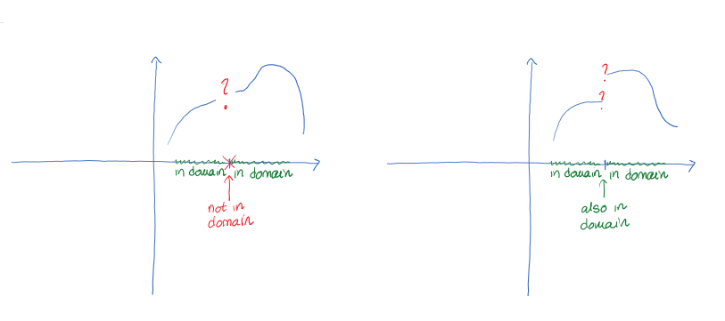
For example, consider the graph below, which illustrates some of the different ways a function can behave at and near a point, and consider the table that contains some numerical information about the function and its behavior.
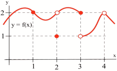
| [latex]a[/latex] | [latex]f(a)[/latex] | [latex]\lim\limits_{x\to a} f(x)[/latex] |
| 1 | 2 | 2 |
| 2 | 1 | 2 |
| 3 | 2 | Does not exist (DNE) |
| 4 | Undefined | 2 |
Based on the information in the table, we can conclude that [latex]f[/latex] is continuous at 1 since [latex]\lim\limits_{x\to 1} f(x) = 2 = f(1)[/latex].
We can also conclude from the information in the table that [latex]f[/latex] is not continuous at 2 or 3 or 4, because [latex]\lim\limits_{x\to 2} f(x) \neq f(2)[/latex], [latex]\lim\limits_{x\to 3} f(x) \neq f(3)[/latex], and [latex]\lim\limits_{x\to 4} f(x) \neq f(4)[/latex].
The behaviors at [latex]x = 2[/latex] and [latex]x = 4[/latex] exhibit a hole in the graph, sometimes called a removable discontinuity, since the graph could be made continuous by changing the value of a single point.
The behavior at [latex]x = 3[/latex] is called a jump discontinuity, since the graph jumps between two values.
So which functions are continuous? It turns out pretty much every function you’ve studied is continuous where it is defined. In particular:
The following types of functions are continuous everywhere on their domain:
- power
- polynomial
- rational
- exponential
- logarithmic
- sine and cosine
- any combination of the above function types
This is extremely helpful in our study of the behaviour of a function because the definition of continuity says that for a continuous function, [latex]\lim\limits_{x\to a} f(x) = f(a)[/latex]. That means for a continuous function, we can find the limit by direct substitution (evaluating the function) if the function is continuous at [latex]a[/latex].
This leads us to a very important note: if we are dealing with a function that is continuous everywhere on its domain, then the only potential "trouble" or "deviation from expected" will come from the input values where the given function is not defined, i.e, at the input values that are not in the domain.
Review video: Continuity
(by Eric Bancroft, licensed under a Creative Commons Attribution-NonCommercial-NoDerivatives 4.0 International License)
Example 7
a. [latex]\lim\limits_{x\to 2} x^3-4x[/latex]
b. [latex]\lim\limits_{x\to 2} \dfrac{x-4}{x+3}[/latex]
c. [latex]\lim\limits_{x\to 2} \dfrac{x^2-4x}{x^2-2x}[/latex]Answer:a. The given function is polynomial, and so it is defined for all values of [latex]x[/latex]. Therefore, we can find the limit by direct substitution:[latex]\lim\limits_{x\to 2} x^3-4x = 2^3-4(2) = 0.[/latex]b. The given function is rational. It is not defined at [latex]x = -3[/latex], but we are taking the limit as [latex]x[/latex] approaches [latex]2[/latex]. Since the function is defined at [latex]x=2[/latex], so we can use direct substitution:[latex]\lim\limits_{x\to 2} \dfrac{x-4}{x+3} = \dfrac{2-4}{2+3}= -\dfrac{2}{5}[/latex]c. This function is not defined at [latex]x=2[/latex] (this value makes the denominator 0), and so is not continuous at [latex]x = 2[/latex]. Therefore, we cannot use direct substitution and have to evaluate the limit using analysis:[latex]\begin{align*} \lim\limits_{x\to 2} \dfrac{x^2-4x}{x^2-2x}&\overset{rewrite}{=}\lim\limits_{x\to 2} \dfrac{x(x-4)}{x(x-2)}\underset{analyze}{\overset{rewrite}{=}}\lim\limits_{x\to 2} \dfrac{\overbrace{x-4}^{\to -2}}{\underbrace{x-2}_{\to 0}}\\\\ &=\dfrac{\text{negative number}}{\text{infinitely small number, but is it negative or positive?}}=\text{cannot answer} \end{align*}[/latex]
Split into cases: evaluate while approaching [latex]0[/latex] from the positive side and evaluate while approaching [latex]0[/latex] from the negative side
[latex]\lim\limits_{x\to 2^+} \dfrac{\overbrace{x-4}^{\to -2}}{\underbrace{x-2}_{\to 0^+}} =\dfrac{\text{negative number}}{\text{infinitely small negative number}}=\infty[/latex]
[latex]\lim\limits_{x\to 2^-} \dfrac{\overbrace{x-4}^{\to -2}}{\underbrace{x-2}_{\to 0^+}} =\dfrac{\text{negative number}}{\text{infinitely small positive number}}=-\infty[/latex]
From this, we can conclude that the function [latex]f(x)=\dfrac{x^2-4x}{x^2-2x}[/latex] has a vertical asymptote at [latex]x=2[/latex], with the function approaching [latex]\infty[/latex] from the left and approaching [latex]-\infty[/latex] from the right.
We conclude this section with a very important theorem, which we will use later as we look for "tops of the hills" and "bottoms of the valleys", i.e., high and low points of a function:
Intermediate Value Theorem
Suppose that [latex]f[/latex] is a continuous function on the closed interval [latex][a, b][/latex] and let [latex]N[/latex] be any number between [latex]f(a)[/latex] and [latex]f(b)[/latex], where [latex]f(a)\neq f(b)[/latex]. Then there exists a number [latex]c\in(a,b)[/latex] such that [latex]f(c)=N[/latex].
Special case: If [latex]f[/latex] is continuous on some closed interval [latex][a, b][/latex] and [latex]f(a)<0[/latex] while [latex]f(b)>0[/latex] (or vice versa), then [latex]f[/latex] has a horizontal intercept, i.e., there is a value [latex]c[/latex] for which [latex]f(c)=0[/latex].
This theorem becomes quite useful in situations where we are looking for zeros of a function but we cannot determine them using the usual tools such as factoring.
For example, we can use Intermediate Value Theorem to demonstrate that [latex]f(x)=4x^3-6x^2+3x-2[/latex] has a zero (an x-intercept) somewhere on the interval [latex](1, 2)[/latex]. This is true because [latex]f(x)[/latex] is a polynomial, and so it is a continuous function on the interval [latex][1, 2][/latex]. Since [latex]f(1)=-1\lt 0[/latex] and [latex]f(2)=12\gt 0[/latex], by the Intermediate Value Theorem there is a value [latex]c\in(1,2)[/latex] such that [latex]f(c)=0[/latex]. Note that we don't know what that value is; we only know that it exists. Later in the course we will learn methods that will allow us to find its approximation, but for that we need the notion of a derivative.
Section Exercises
Work on the following exercises. Discuss your solutions with your peers and/or course instructor.
IC4NITS Exercises 2.1 - Limits and Continuity
