1.5 Transcendental Functions: Exponential, Logarithmic, and Trigonometric Functions
1.5 Transcendental Functions: Exponential, Logarithmic, and Trigonometric Functions
Transcendental functions are functions that transcend, i.e., go beyond, the algebraic functions. They are the functions that cannot be expressed as a finite sequence of algebraic operations. In other words, transcendental functions cannot be represented through a series of calculations. Their output values are defined through the input values using rules that are abstractly defined using some concept and the relationships arising from that concept. For example, the trigonometric functions sine and cosine are defined through the relationships that can be built using a unit circle (a circle of radius 1).
Most important transcendental functions are exponential functions, logarithmic functions, trigonometric functions and inverse trigonometric functions. In this section we will discuss the first three (we will not discuss the inverse trigonometric functions).
Exponential functions
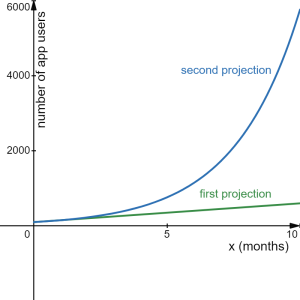
Consider these two potential projections on the number of users of an app over time:
- The app currently has 100 users, and its user base grows by 50 users each month.
- The app currently has 100 users, and its user base grows by 50% each month.
The first projection is based on linear growth. In linear growth, we have a constant rate of change – a constant number that the output increased for each increase in input. In the first projection, the number of new users per month is the same each month.
The second projection is different – we have a constant percent rate of change in users per month rather than a constant number of users/month as our rate of change. A rate of change that is characterized by a constant percent rate of change gives rise to exponential growth. To see the significance of this difference, compare a 50% increase when there are 100 users to a 50% increase when there are 1000 users:
- With 100 app users, a 50% increase is 50 new users over the next month.
- With 1000 app users, a 50% increase is 500 new users during the next month.
Calculating the number of app users after several months, we can clearly see the difference in results.
| Months | First projection (linear) | Second projection (exponential) |
| 2 | 200 | 225 |
| 4 | 300 | 506 |
| 6 | 400 | 1139 |
| 8 | 500 | 2563 |
| 10 | 600 | 5767 |
Terminology of exponential functions
An exponential growth or decay function is a function that grows or shrinks at a constant percent growth or decay rate. The equation can be written in the form
[latex]f(x)=f_0(1+r)^x[/latex]
or
[latex]f(x)=f_0\cdot b^x[/latex] where [latex]b=1+r[/latex]
Here:
- [latex]f_0[/latex] is the initial or starting value of the function,
- [latex]r[/latex] is the percent growth or decay rate, written as a decimal (note that [latex]r[/latex] is a negative number in the case of rate of decay),
- [latex]b[/latex] is the growth factor or growth multiplier. Since powers of negative numbers sometimes exist and sometimes do not, we limit [latex]b[/latex] to positive values.
Important note: Both the exponential functions and the power functions involve expressions with an exponent on a base. However, the two types of functions are fundamentally different in their characteristics and their behaviour, and therefore you must be able to differentiate between them. You can do so by noting that:
a power function has the variable in the base (and the exponent is a constant number)
an exponential function has the variable in the exponent (and the base is a constant number)
Example 1 - Exponential Growth
India’s population was 1.14 billion in the year 2008 and is growing by about 1.34% each year. Write an exponential function for India’s population, and use it to predict the population in 2020.
Answer: population of India as a function of time? population prediction for 2020?
population of India as a function of time:
First, let's determine the details of the independent and the dependent variable. Since the population size is a function of time, the population size is the dependent variable and the time is the independent variable. Let [latex]P[/latex] be the size of India's population, measured in billions. Since our initial data point is in year 2008, let the time [latex]t[/latex] represent the number of years since 2008.
If the population is growing exponentially, then the general formula for our function would be
[latex]P(t)=P_0(1+r)^t[/latex]
where [latex]P_0[/latex] is the initial population size and [latex]r[/latex] is the annual percent change in the population size.
Using 2008 as our starting time ([latex]t = 0[/latex]), our initial population will be 1.14 billion and so [latex]P_0=1.14[/latex]. Since the percent growth rate was 1.34%, we have [latex]r=0.0134[/latex]. Therefore,
[latex]P(t)=1.14(1+0.0134)^{t}[/latex]
population prediction for 2020:
To estimate the population in 2020, we evaluate the function at [latex]t = 12[/latex], since 2020 is 12 years after 2008:
[latex]P(t)=1.14(1+0.0134)^{12}\approx 1.337[/latex]
Therefore, the projected population size of India using this model would be 1.337 billion people.
(How does that compare to what India's population was in 2020? Was this a reasonable model?)
Example 2 - Exponential Decay
A cell phone company is introducing to the market a new model for a cell phone and needs to plan how long they should keep manufacturing and selling the current model before taking it off the market. Market analysis and the analysis of their sales trends with their "old" models suggests that the sales of the current model will decrease by 12.34% annually, while their current sales are at 259.37 million. Create the function model that represents the number of current model cell phones sold (in millions) each year, call it [latex]n[/latex], after [latex]t[/latex] years from now, and estimate the annual sales of the current models 5 years from now.
Answer: [latex]n(t)=?, n(5)=?[/latex] where [latex]n[/latex] decreasing by % per year [latex]\rightarrow[/latex] exponential decay
Hence, the number of phones sold each year is 100%-12.34%=87.66% of the number of phones sold the previous year. In addition, their sales were 259.37 million at the start. Therefore, we have:
[latex]\begin{align*} n(0)&=259.37\\ n(1)&=n(0)\cdot (1-0.1234)=259.37(0.8766)\\ n(2)&=n(1)\cdot(1-0.1234)=259.37(0.8766)(0.8766)\\ &=259.37(0.8766)^2\\ n(3)&=n(2)\cdot(1-0.1234)=259.37(0.8766)^2(0.8766)\\ &=259.37(0.8766)^3\\ \vdots& \end{align*}[/latex]
Therefore, [latex]n(t)=259.37(0.8766)^t,\quad t\ge 0[/latex].
In particular, five years from now, [latex]t=5[/latex], and so
[latex]n(5)=259.37(0.8766)^5\approx 134.25[/latex]
Therefore, five years from now, the annual sales of the current model would be approximately 134.25 million.
Important note: how to distinguish between linear and exponential change?
If a quantity is changing by a fixed amount over equal periods, the change is linear.
If a quantity is changing by a percentage rate over equal periods, the change is exponential.
Example 3 - interpreting components of an exponential function
Suppose that
[latex]T(q)=86(1.64)^q[/latex]
represents the total number of Android smart phone contracts, in thousands, held by a certain Verizon store region and measured quarterly since January 1, 2015. Interpret all of the parts of the equation for [latex]T(q)[/latex] and briefly explain the meaning of
[latex]T(2)=86(1.64)^2=231.3056[/latex]
Answer: Meaning of parts of [latex]T(q)[/latex]? Meaning of [latex]T(2)=231.3056?[/latex]
Meaning of parts of [latex]T(q)[/latex]:
According to its definition, [latex]T(q)[/latex] represents the total number of Android smart phone contracts, in thousands, [latex]q[/latex] quarters since January 1, 2015. By analyzing the rule for calculating [latex]T(q)[/latex], we can see that it is an exponential function, with 86 as our initial value. This means that on Jan. 1, 2015 this region had 86,000 Android smart phone contracts.
Since the growth factor is [latex]b = 1 + r = 1.64[/latex], we have that [latex]r=0.64[/latex], and so we know that every quarter the number of smart phone contracts grows by 64%.
Meaning of [latex]T(2)=231.3056[/latex]:
Considering [latex]T(2)[/latex], we know that it represents the total number of Android smart phone contracts, in thousands, held by the given Verizon store region after [latex]2[/latex] quarters, i.e., after 6 months. Therefore, [latex]T(2) = 231.3056[/latex] means that at the end of the second quarter there were approximately 231,306 Android smart phone contracts.
Euler's number
When working with exponentials, there is a special constant we must talk about. It is the constant [latex]e[/latex], called Euler's number. This number has a special place in describing many phenomena in mathematics. It can be used whenever we wish to model any type of continuous growth or decay. Just like pi, or [latex]\pi[/latex], it has infinitely many non-repeating decimals and it is an irrational number, meaning it cannot be represented as a fraction. Your calculator will use different number of decimals to round [latex]e[/latex] to an approximate value, depending on your calculator settings, however typically we would approximate it as follows:
Euler’s Number:
[latex]e\approx 2.718282[/latex]
For those who are interested, note that the value of [latex]e[/latex] is calculated by increasing the value of [latex]n[/latex] towards infinity in the following expression:
[latex]e=\left(1+\frac{1}{n}\right)^n\text{ as }n\to\infty[/latex]
You can try it out yourself by calculating the above expression for increasingly larger values of [latex]n[/latex]. If you are familiar with the concept of compound interest, note also that this is the same calculation as the growth portion of a periodic compounded interest where the annual rate is 100% and the frequency of compounding approaches infinite times per year.
Because [latex]e[/latex] is often used as the base of an exponential function, most scientific and graphing calculators have a key that can calculate powers of [latex]e[/latex], usually labeled [latex]e^x[/latex]. Some computer software instead defines a function exp(x), where
exp(x) = [latex]e^x[/latex]. Since calculus studies continuous change, we will almost always use the [latex]e[/latex]-based form of exponential equations in this course.
Continuous Growth Formula
Continuous growth can be calculated using the formula [latex]f(x)=ae^{kx}[/latex] where
- [latex]a[/latex] is the starting amount,
- [latex]k[/latex] is the continuous growth rate.
It turns out that every exponential function [latex]f(x)=ab^x[/latex] can be written as a horizontal stretch/shrink of a continuous growth (or decay) function, specifically, it can be written as [latex]f(x)=ae^{kx}[/latex] for some value [latex]k[/latex]. We will discuss this later in this section when we discuss logarithms and logarithmic functions.
Graphs of exponential functions
Graphical features of exponential functions
Graphically, in the function [latex]f(x)=a\cdot b^x[/latex]:
- [latex]a[/latex] is the vertical intercept of the graph.
- [latex]b[/latex] determines the rate at which the graph grows:
- the function will increase if [latex]b \gt 1[/latex],
- the function will decrease if [latex]0 \lt b \lt 1[/latex].
- The graph will have a horizontal asymptote at [latex]y = 0[/latex].
- The graph will be concave up if [latex]a \gt 0[/latex]; concave down if [latex]a \lt 0[/latex].
- The domain of the function is all real numbers.
- The range of the function is [latex](0,\infty)[/latex] if [latex]a \gt 0[/latex], and [latex](-\infty, 0)[/latex] if [latex]a \lt 0[/latex].
When sketching the graph of an exponential function, it can be helpful to remember that the graph will pass through the points [latex](0, a)[/latex] and [latex](1, ab)[/latex].
The base value [latex]b[/latex] will determine the function’s behavior as the input values approach positive or negative infinity:
- If [latex]b \gt 1[/latex], as [latex]x\to\infty[/latex], [latex]b^x\to\infty[/latex], and as [latex]x\to -\infty[/latex], [latex]b^x\to 0[/latex].
- If [latex]0 \lt b \lt 1[/latex], as [latex]x\to\infty[/latex], [latex]b^x\to 0[/latex], and as [latex]x\to -\infty[/latex], [latex]b^x\to \infty[/latex].
Helpful hint: reread the above two descriptions of the behaviour of [latex]b^x[/latex] by reading the arrows [latex]\to[/latex] as "approaches". The meaning of the symbols and thus the description of the behaviour of the function will then make more sense. As a note of things to come, the word "approaches" and thus the symbol "[latex]\to[/latex]" will form a foundation of our study of calculus.
Example 4 - sketching graphs of exponential functions
Sketch a graph of [latex]f(x)=4\left(\frac{1}{3}\right)^x[/latex]
Answer: graph of [latex]f(x)[/latex]?
This graph will have a vertical intercept at (0,4), and pass through the point [latex]\left(1,\frac{4}{3} \right)[/latex]. Since [latex]b \lt 1[/latex], the graph will be decreasing towards zero. Since [latex]a \gt 0[/latex], the graph will be concave up.
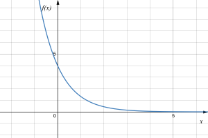
We can also see from the graph the long run behavior: as [latex]x\to\infty[/latex], [latex]f(x)\to 0[/latex], and as [latex]x\to -\infty[/latex], [latex]f(x)\to \infty[/latex].
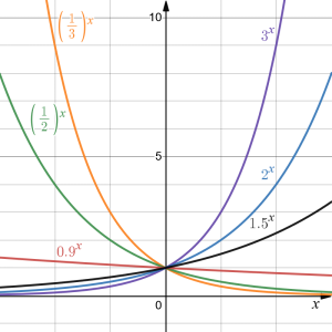
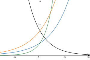
To get a better feeling for the effect of [latex]a[/latex] and [latex]b[/latex] on the graph, examine the sets of graphs below. The first set shows various graphs, where [latex]a[/latex] remains the same and we only change the value for [latex]b[/latex]. Notice that the closer the value of [latex]b[/latex] is to 1, the less steep the graph will be.
In the next set of graphs, [latex]a[/latex] is altered and our value for [latex]b[/latex] remains the same.
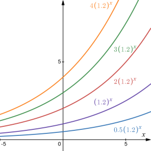
Notice that changing the value for [latex]a[/latex] changes the vertical intercept. Since [latex]a[/latex] is multiplying the [latex]b^x[/latex] term, [latex]a[/latex] acts as a vertical stretch factor, not as a shift. Notice also that, for all of these functions, the behavior of the function as the input approaches [latex]\pm \infty[/latex] is the same because the growth factor did not change and none of these [latex]a[/latex] values introduced a vertical flip.
Example 5 - determining the graphs of exponential functions based on initial value and growth factor
 Match each equation with its graph.
- [latex]f(x)=2(1.3)^x[/latex]
- [latex]g(x)=2(1.8)^x[/latex]
- [latex]h(x)=4(1.3)^x[/latex]
- [latex]k(x)=4(0.7)^x[/latex]
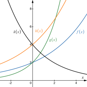 Answer:
The graph of [latex]k(x)[/latex] is the easiest to identify, since it is the only equation with a growth factor less than one, which will produce a decreasing graph.
The graph of [latex]h(x)[/latex] can be identified as the only growing exponential function with a vertical intercept at [latex](0,4)[/latex].
The graphs of [latex]f(x)[/latex] and [latex]g(x)[/latex] both have a vertical intercept at [latex](0,2)[/latex], but since [latex]g(x)[/latex] has a larger growth factor, we can identify it as the graph increasing faster.
Logarithmic functions
Logarithmic functions arise from logarithms, which are the inverse of exponential expressions where the unknown variable is in the exponent. In the networking and IT security area, logarithmic functions, together with exponential functions, are widely used in analyzing digital transmissions.
Review of logarithms
Logarithms allow us to solve equations where the variable is in the exponent. They are also commonly used to express quantities that vary widely in size. For example, see the New York Times article on how the logarithmic scale charts were used to visualise the spread of the Covid-19 virus in the early 2020s: A Different Way to Chart the Spread of Coronavirus.
Logarithm as an inverse equivalent to an exponential
The logarithm (base [latex]b[/latex]) function, written [latex]\log_b (x)[/latex], is the inverse of the exponential function (base [latex]b[/latex]), [latex]b^x.[/latex] This means the statement [latex]b^p=q[/latex] is equivalent to the statement [latex]\log_b (q)=p[/latex].
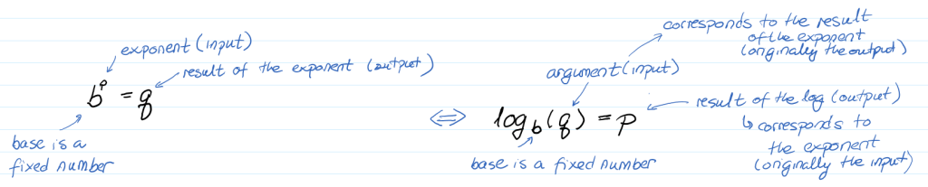
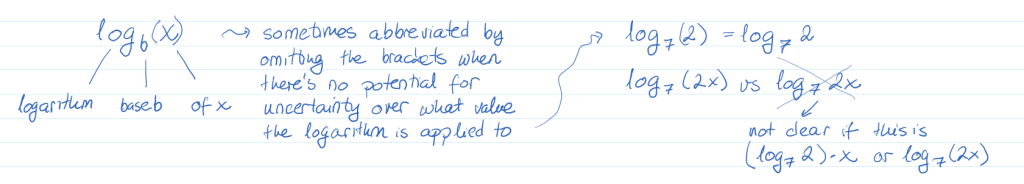
We read these symbols, [latex]\log_b (x)[/latex], as logarithm base b of x or, abbreviated, as log base b of x. Do not read as "log(arithm) b x" - the words base and of tell us very important information on the role that the values we are using in this expression are playing.
Sometimes we abbreviate by omitting the parentheses around the input variable (also called the argument) but have to be careful in that to ensure that there is no possibility of confusion over what the argument (i.e., the input variable) is.
Example 6
Write these exponential equations as logarithmic equations:
- [latex]2^3=8[/latex]
- [latex]5^2=25[/latex]
- [latex]10^{-4}=\frac{1}{10000}[/latex]
Answer:
- [latex]2^3=8[/latex] is equivalent to [latex]\log_2(8)=3[/latex].
- [latex]5^2=25[/latex] is equivalent to [latex]\log_5(25)=2[/latex].
- [latex]10^{-4}=\frac{1}{10000}[/latex] is equivalent to [latex]\log_{10}\left(\frac{1}{10000}\right)=-4[/latex].
Example 7
Answer: By rewriting this equation using a logarithm, we get [latex]x=\log_2(10)[/latex].
If you consider the last example, while [latex]x=\log_2(10)[/latex] does define a solution, and an exact solution at that, you may find it somewhat unsatisfying since it is difficult to compare this expression to the exact values it represents. Also, giving an exact expression for a solution is not always useful - often we really need a decimal approximation to the solution, particularly if we are working with logarithms within some real-world context, as in in the context of money or size or a number of people etc. Luckily, this is a task calculators and computers are quite adept at. Unluckily for us, most calculators and computers will only evaluate logarithms of two bases: base 10 and base [latex]e[/latex]. Happily, this ends up not being a problem, as we’ll see briefly.
Common and natural logarithms and the change of base formula
We introduce the definition and the notation for two most widely used logarithm bases, each of which can, in turn, be used to determine values of logarithms on any other base.
The common log is the logarithm with base 10, and is typically written [latex]\log(x)[/latex]. Specifically, instead of writing [latex]\log_{10}(x)[/latex] we can write, for short, [latex]\log(x)[/latex]. In other words, when no base is written, by convention it is implied that the base is 10.
The natural log is the logarithm with base [latex]e[/latex], and is typically written [latex]\ln(x)[/latex]. Specifically, instead of writing [latex]\log_{e}(x)[/latex] we can write, for short, [latex]\ln(x)[/latex]. We read this sounding as "lawn of x" (as in mowing the lawn).
We can then use the change of base formula and the common calculator logarithm calculation keys log and ln to calculate the values of a logarithm on any base:
[latex]\log_b(x)=\dfrac{\log_c(x)}{\log_c(b)}=\dfrac{\log(x)}{\log(b)}=\dfrac{\ln(x)}{\ln(b)}[/latex]
Example 8
Evaluate [latex]\log(1000)[/latex] without a calculator by using the definition of the common log.
Answer: [latex]\log(1000)[/latex]?, using the definition
To evaluate [latex]\log(1000)[/latex], we can say [latex]x=\log(1000)[/latex], then rewrite into exponential form using the common log base of 10:
[latex]10^x=1000[/latex]
Using our general knowledge, we should recognize that 1000 is the cube of 10, i.e., [latex]10^3=1000[/latex]. Hence, [latex]x = 3[/latex].
We also can use the inverse property of logs to write [latex]\log_{10}\left(10^3\right) =3[/latex].
| Number | Number as exponential | log(number) |
| 1000 | [latex]10^3[/latex] | 3 |
| 100 | [latex]10^2[/latex] | 2 |
| 10 | [latex]10^1[/latex] | 1 |
| 1 | [latex]10^0[/latex] | 0 |
| 0.1 | [latex]10^{-1}[/latex] | -1 |
| 0.01 | [latex]10^{-2}[/latex] | -2 |
| 0.001 | [latex]10^{-3}[/latex] | -3 |
Example 9
Answer: Using a computer or calculator, we can evaluate and find that [latex]\log(500)\approx 2.69897[/latex].
Example 9
Evaluate [latex]\log(500)[/latex] using you calculator or computer.
Answer: [latex]\log(500)[/latex]? use calculator
Using a computer or calculator, we can evaluate and find that [latex]\log(500)\approx 2.69897[/latex].
Because logarithms are inverse functions of exponentials, we can, in particular, use them to solve exponential equations, where the unknown is in the exponent, in much the same way as we use the inverse properties of addition vs. subtraction or multiplication vs. division when rearranging equations to solve for an unknown value. For this, we need to know some fundamental properties of logarithms.
Properties of Logarithms
Inverse Properties:
[latex]\log_b(b^x)=x\quad (1)[/latex]
[latex]b^{\log_b(x)}=x\quad (2)[/latex]
Exponent Property
[latex]\log_b\left(x^k\right)=k\cdot\log_b(x)\quad (3)[/latex]
Here is an example how these properties are useful:
Suppose we have the following equation and are asked to determine the value of [latex]x[/latex]:
[latex]2\cdot 1.8^x=17.2[/latex]
To solve for [latex]x[/latex], we first have to determine which operations, and in which order, are acting on [latex]x[/latex], and then undo the operations in the opposite order. Because [latex]x[/latex] is first placed into the exponent of 1.8, and then the new value is multiplied by 2, the last operation was "multiply by 2" and so we first have to undo the last operation, i.e., we must divide by 2, on both sides of the equation (to maintain the balance of the left and the right side):
[latex]1.8^x=\frac{17.2}{2}[/latex]
Looking at the equation now, we can see that the only operation affecting [latex]x[/latex] is that [latex]x[/latex] is placed into the exponent of 1.8. The opposite operation of "placing a value into the exponent" would be the inverse property (1), so we could apply [latex]\log_{1.8}[/latex] to get just [latex]x[/latex]. However, the typical scientific calculator only calculates the common and the natural log, so [latex]\log_{1.8}[/latex] won't be helpful when applied to the other side of the equation. So instead we will apply either [latex]\log[/latex] or [latex]\ln[/latex] to both sides of the equation, and then bring down the exponent, where our unknown is, by using the exponent property (3):
[latex]\begin{align*} \ln(1.8)^x&=\ln\left(\frac{17.2}{2}\right)\Rightarrow x\cdot \ln(1.8)=\ln\left(\frac{17.2}{2}\right)\\ &\Rightarrow x=\frac{\ln\left(\frac{17.2}{2}\right)}{\ln(1.8)}\approx 3.660788 \end{align*}[/latex]
General process for solving exponential equations using logarithms
- Isolate the exponential expressions when possible.
- Take the logarithm of both sides.
- Utilize the exponent property for logarithms to pull the variable down from the exponent.
- Continue to use algebra to solve for the variable.
Example 10 - solving for a variable in the exponent
In a previous example, we predicted the population (in billions) of India [latex]t[/latex] years after 2008 by using the function
[latex]P(t)=1.14(1+0.0134)^t[/latex]
If the population continues following this trend, when will the population reach 2 billion?
Answer: [latex]t =?[/latex] where [latex]P(t) = 2[/latex] and [latex]P(t)=1.14(1+0.0134)^t=1.14(1.0134)^t[/latex]
| State the initial equation and note that the last operation affecting the variable is multiplication by 1.14. | [latex]1.14(1.0134)^t=2[/latex] |
| Divide by 1.14 on both sides to undo the last operation and note that the last operation now is the placement of t into the exponent. | [latex]\Rightarrow 1.0134^t=\frac{2}{1.14}[/latex] |
| Apply the common log to both sides to undo the last operation and note that our variable is now in the exponent of the argument of a logarithm. | [latex]\Rightarrow \log\left(1.0134^t\right)=\log\left(\frac{2}{1.14}\right)[/latex] |
| Use the exponent property for logs (3) to bring down the exponent that is inside the log by multiplying it with the logarithm and note that the last operation now is multiplication by log(1.0134). | [latex]\Rightarrow t\cdot \log(1.0134)=\log\left(\frac{2}{1.14}\right)[/latex] |
| Divide both sides by ln(1.0134) to undo the last operation. Note that there are no more operations taking place on the variable. | [latex]\Rightarrow t = \dfrac{\log\left(\frac{2}{1.14}\right)}{\log(1.0134)}[/latex] |
| Calculate. | [latex]\Rightarrow t\approx 42.23 \text{ years}[/latex] |
If this growth rate continues, the model predicts the population of India will reach 2 billion about 42 years after 2008, or approximately in the year 2050.
Note that in the process of solving the equation we used the common logarithm [latex]\log[/latex] to bring the exponent down. We also could have used the natural logarithm [latex]\ln[/latex] or, for that matter, logarithm with any (positive) base - the final result would have been the same.
Example 11 - solving for a variable in the exponent
Solve [latex]5e^{-0.3t}=2[/latex] for [latex]t[/latex].
Answer:
| State the initial equation and note that the last operation affecting the variable is multiplication by 5. | [latex]5e^{-0.3t}=2[/latex] |
| Divide by 5 on both sides to undo the last operation and note that the last operation now is the placement of -0.3t into the exponent. | [latex]\Rightarrow e^{-0.3t}=\frac{2}{5}[/latex] |
| Apply the natural log to both sides to undo the last operation and note that our variable is now in the exponent of the argument of a logarithm. | [latex]\Rightarrow \ln\left(e^{-0.3t}\right)=\ln\left(\frac{2}{5}\right)[/latex] |
| Use the exponent property for logs (3) to bring down the exponent that is inside the log by multiplying it with the logarithm and note that the last operation now is multiplication by -0.3 ln(e). | [latex]\Rightarrow {-0.3t}\cdot \ln\left(e\right)=\ln\left(\frac{2}{5}\right)[/latex] |
| Use the inverse property for logs (2) to simplify the equation and note that the last operation now is multiplication by -0.3. | [latex]\Rightarrow -0.3t=\ln\left(\frac{2}{5}\right)[/latex] |
| Divide both sides by -0.3 to undo the last operation. Note that there are no more operations taking place on the variable. | [latex]\Rightarrow t = \dfrac{\ln\left(\frac{2}{5}\right)}{-0.3}[/latex] |
| Calculate. | [latex]\Rightarrow t\approx 3.054[/latex] |
Note that in the process of solving the equation we used the natural logarithm [latex]\ln[/latex] to bring the exponent down. We also could have used the common logarithm [latex]\log[/latex] or, for that matter, logarithm with any (positive) base - the final result would have been the same.
Functions defined through a logarithm
A function of the form [latex]f(x)=\log_b(x)[/latex] is called a logarithmic function. Because of the properties of logarithms and their relationships to exponential expressions, logarithmic functions are the inverse of exponential functions and vice versa. This is reflected through the characteristics of logarithmic functions as, in a way, the opposite of the characteristics of exponential functions, through a reversal of the relationship between the input and the output.
Graphical features of the logarithm
Graphically, given the function [latex]g(x)=\log_b(x)[/latex].
- The graph has a horizontal intercept at [latex](1, 0)[/latex].
- The graph has a vertical asymptote at [latex]x = 0[/latex].
- The graph is increasing and concave down.
- The domain of the function is [latex]x \gt 0[/latex], or [latex](0, \infty)[/latex] in interval notation.
- The range of the function is all real numbers, or [latex](-\infty, \infty)[/latex] in interval notation.
Here are a couple of examples of the "reversal" in the characteristics between the exponential and the logarithmic function:
The basic exponential function [latex]b^x[/latex] passes through the point [latex](0,1)[/latex] whereas the basic logarithmic function [latex]\log_bx[/latex] passes through the point [latex](1,0)[/latex].
The basic exponential function [latex]b^x[/latex] approaches [latex]0[/latex] from the positive side as [latex]x[/latex] approaches [latex]-\infty[/latex] whereas the basic logarithmic function [latex]\log_bx[/latex] approaches [latex]-\infty[/latex] as [latex]x[/latex] approaches [latex]0[/latex] from the positive side. Specifically, the basic exponential function has a horizontal asymptote while the basic logarithmic function has a vertical asymptote.
You can see this symmetry of characteristics graphically here: exponential function vs logarithmic function. You can change the value of the base using the base parameter slider.
When sketching a general logarithm with base [latex]b[/latex], it can be helpful to remember that the graph will pass both through [latex](1, 0)[/latex] and [latex](b, 1)[/latex].
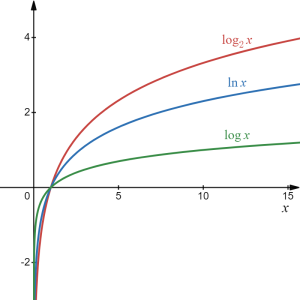
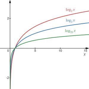
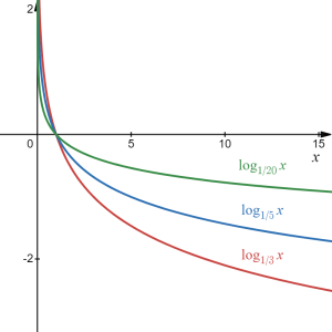
To get a feeling for how the base affects the shape of the graph, examine the graphs below:
 |
 |
 |
Example 12 - domain of a logarithmic function
Find the domain of the function [latex]f(x)=\log(5-2x)[/latex].
Answer: domain of [latex]f(x)[/latex]? [latex]\to[/latex] all input values that produce an output value
input values: x?
output value: [latex]f(x)=\log(5-2x)[/latex]
The logarithm is only defined when the input is positive, so this function will only be defined when [latex]5-2x \gt 0[/latex]. Solving this inequality, [latex]-2x \gt -5[/latex], so [latex]x\lt \frac{5}{2}[/latex]. Therefore, the domain of this function is [latex]\left\{x\in\mathbb{R}|x\lt \frac{5}{2}\right\}[/latex] or, in interval notation, [latex]\left(-\infty, \frac{5}{2} \right)[/latex].
Trigonometric functions
There is much to be said about trigonometric functions, which play a massive role in mathematical analysis at a higher level than introductory calculus. They are fundamental to complex analysis and are also constituent parts in Fourier series and Fourier transforms, key to signal processing, for example.
Although Fourier transforms are way beyond what we will discuss in this introductory calculus class, you may find the following explanation interesting, and perhaps even fascinating: But what is the Fourier Transform? A visual introduction. If you watch this video, you will recognize, even at our fundamental level, some of the concepts and processes we've discussed so far - concept of a function, how it is is represented, what it means to add two functions and how we can decompose functions into sums of multiple functions (or any other combination of algebraic operations on functions). As you watch this video you will also notice a reference to a transformation along the horizontal ("wrapping a signal faster or slower") and may also note what we said how mathematically things work counterintuitively when we are transforming horizontally.
But we digress. Let's get back to trigonometric functions.
Basic trigonometric functions
The two basic trigonometric functions are the sine function and the cosine function, denoted by [latex]\sin[/latex] and [latex]\cos[/latex], respectively. They arise from the relationships along a unit circle (a circle of radius 1) using the basic properties of right angle triangles, including the relationships between the angles and the relationships between the lengths of the sides of a right angle triangle via the Pythagorean Theorem.
Given an input value [latex]x[/latex], the symbols used to denote the values of the sine and the cosine function are [latex]\sin(x)[/latex] and [latex]\cos(x)[/latex], read as "sine of x" and "cosine of x", respectively. As with the logarithmic function, we can omit the parentheses around the argument (i.e., the input) but only when there is no possibility of uncertainty about what the argument is.
So how are the values of [latex]\sin x[/latex] and [latex]\cos x[/latex] defined, given some value [latex]x[/latex]?
Consider the unit circle centered at the origin (i.e., a circle centered at the point (0,0), with radius 1). We define the values of the sine and the cosine using as the input the length of the arc created from the horizontal axis and going counterclockwise along the circle. The coordinates of the point where the arc ends determine the values of the two functions. In particular, given a unit circle arc length, the value of the first coordinate represents the value of the cosine and the value of the second coordinate represents the value of the sine. See below for an illustration:
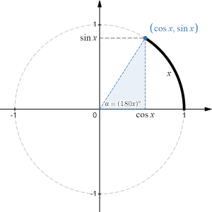
Although there are many trigonometric identities, i.e., equations involving [latex]\sin x[/latex] and [latex]\cos x[/latex], we will not be needing them in this course except, perhaps, the fundamental trigonometric identity arising from Pythagora's Theorem on the unit circle:
[latex]\sin^2 x+\cos^2 x=1[/latex]
Note that, in the above, [latex]\sin^2 x[/latex] means [latex](\sin x)^2[/latex] and [latex]\cos^2 x[/latex] means [latex](\cos x)^2[/latex].
Remember also that both [latex]\sin x[/latex] and [latex]\cos x[/latex] can be calculated by thinking of [latex]x[/latex] as the unit circle arc length (measured in radians) and as the angle at the origin corresponding to the arc (measured in degrees). However, when using a calculator to determine the specific value of a trigonometric function, we have to indicate the input variable units either as radians or degrees. In this course we will work exclusively with the radian units. Thus, you should make sure that your calculator settings are in radians (typically this is displayed in the calculator window using the letter R, as opposed to D or G, the latter representing gradians, with one grad representing 1/400 of the circumference of a circle or, equivalently, one hundredth of the right angle).
Though there is no algebraic formula to calculate the value of sine or cosine, there are some well known input-output pairs, as you will likely recall:
| [latex]x[/latex] (radians) | [latex]\sin x[/latex] | [latex]\cos x[/latex] |
| [latex]0[/latex] | [latex]0[/latex] | [latex]1[/latex] |
| [latex]\frac{\pi}{6}[/latex] | [latex]\frac{1}{2}[/latex] | [latex]\frac{\sqrt{3}}{2}[/latex] |
| [latex]\frac{\pi}{4}[/latex] | [latex]\frac{\sqrt{2}}{2}[/latex] | [latex]\frac{\sqrt{2}}{2}[/latex] |
| [latex]\frac{\pi}{3}[/latex] | [latex]\frac{\sqrt{3}}{2}[/latex] | [latex]\frac{1}{2}[/latex] |
| [latex]\frac{\pi}{2}[/latex] | [latex]1[/latex] | [latex]0[/latex] |
The exact value of [latex]\pi[/latex] cannot be calculated. However, a certain number of digits is programmed into your calculator so that it can perform trigonometric and other calculations involving [latex]\pi[/latex]. For an interesting trip down the story of how [latex]\pi[/latex] came to be and its connection to, among other things, cybersecurity, see: A Brief History of Pi.
Some other properties of the sine and the cosine functions are:
| [latex]\sin x[/latex] | [latex]\cos x[/latex] |
| domain: all real numbers | domain: all real numbers |
| range: [latex][-1, 1][/latex] | range: [latex][-1, 1][/latex] |
| periodic: values repeat in [latex]2\pi[/latex]-periods | periodic: values repeat in [latex]2\pi[/latex]-periods |
| symmetric in the origin | symmetric in the vertical axis |
| odd function: [latex]\sin(-x)=-\sin(x)[/latex] | even function: [latex]\cos(-x)=\cos(x)[/latex] |
Graphically they can be represented as follows:
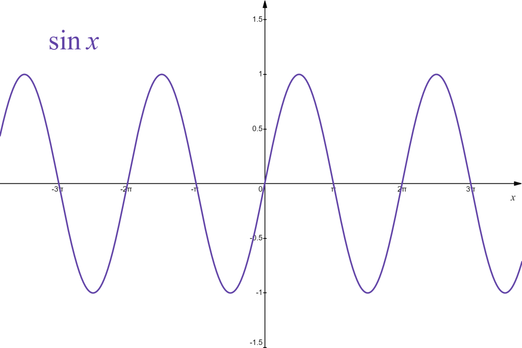 |
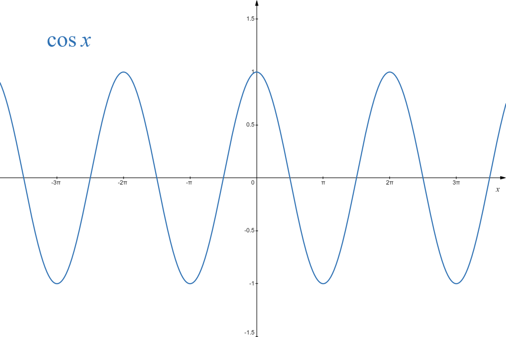 |
Other types of trigonometric functions
There are other commonly used trigonometric functions, defined through algebraic operations on the sine and the cosine functions. You should know them:
| tangent: | [latex]\tan x=\frac{\sin x}{\cos x}[/latex] |
| cotangent: | [latex]\cot x=\frac{\cos x}{\sin x}[/latex] |
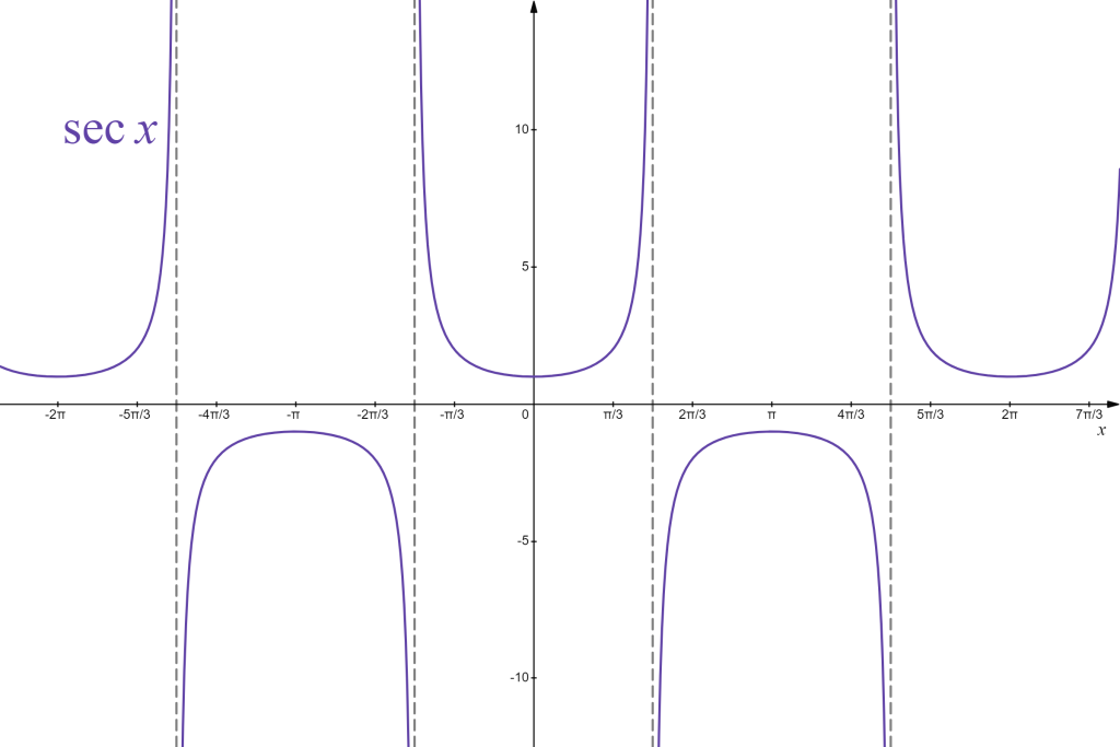
| secant: | [latex]\sec x=\frac{1}{\cos x}[/latex] |
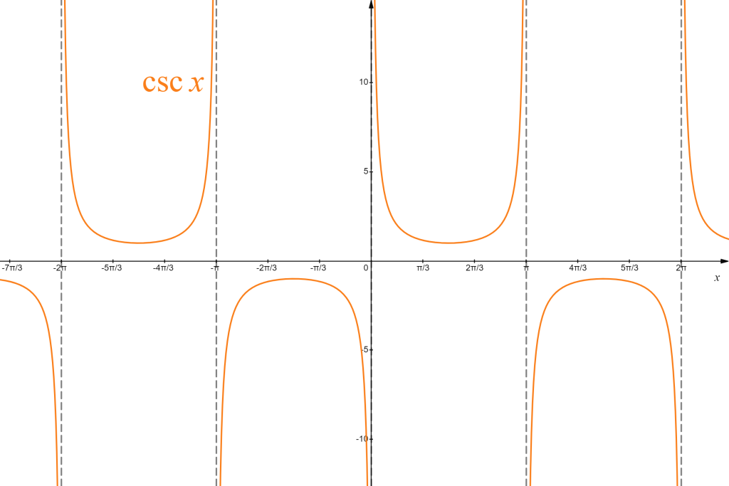
| cosecant: | [latex]\csc x=\frac{1}{\sin x}[/latex] |
Since they are built from cosine and sine, these functions also exhibit periodic behaviour and symmetries. However, since they involve division, their domains are restricted to divisor (denominator) not being equal to zero, graphically giving rise to infinitely many vertical asymptotes, repeated periodically. Their ranges vary, with the range of tangent and cotangent being all real numbers, and the range of secant and cosecant being all real numbers, excluding [latex](-1,1)[/latex]. They can be represented graphically as follows:
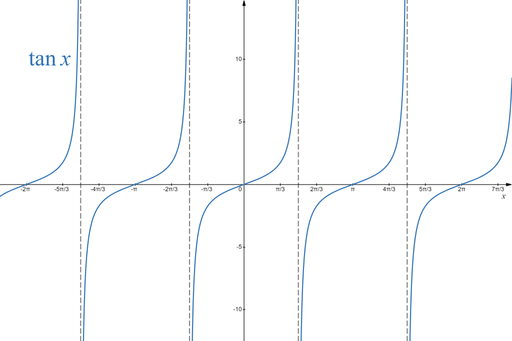 |
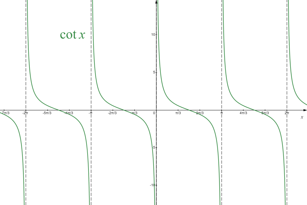 |
 |
 |
Section Exercises
Work on the following exercises. Discuss your solutions with your peers and/or course instructor.
Exercises 1.5 - Transcedental Functions
