1.4 Algebraic functions: Polynomial and Rational Functions
1.4 Algebraic functions: Polynomial and Rational Functions
Algebraic functions
Although a more precise and more general definition for algebraic functions exists, for the purposes of our course we will say that algebraic functions are functions that can be built from a finite number of algebraic operations applied to the input variable. In other words, they are the functions that can be represented by formulas using only the algebraic operations such as addition, subtraction, multiplication, division, and raising to a fractional exponent.
For example,
[latex]m(p)=\frac{3 \sqrt[5]{p-17}}{2 p^2}[/latex]
is an algebraic function because it only involves algebraic operations on the input variable [latex]p[/latex]. In case the fifth root confuses you, recall that a root of some value is also considered as that value raise to the root reciprocal, i.e., [latex]\sqrt[n]{x}=x^{1/n}[/latex]. In other words, a root is effectively a value raised to a fractional exponent.
On the other hand, the function
[latex]k(p)=\frac{3 \sqrt[5]{p-17}}{2 \cos{p}}[/latex]
is not an algebraic function because, although it involves algebraic operations, it also involves the application of the cosine function on the input variable, which is not an algebraic operation.
Power functions
The simplest algebraic functions are the power functions with rational exponents (i.e., exponents that can be written as a fraction), along with their slight generalization to the constant multiple of a power function.
A power function is a function involving a base and an exponent, as in [latex]x^k[/latex], where [latex]x[/latex] is the variable and [latex]k[/latex] is some constant.
Note that a power function has the variable in the base of the expression. This is different from, for example, the exponential function (to be discussed in the next section), say [latex]k^x[/latex], where the variable is in the exponent. Being able to distinguish between power functions and exponential functions will be key throughout our calculus journey.
Although you may not have used this terminology before, you are familiar and have worked with power functions before. For example, [latex]x,\ x^2,\ p^5,\ m^{-7},\ x^{0.671}[/latex], etc. are all power functions because they involve a base and an exponent, where the variable is in the base. (Remember that [latex]x[/latex] is, by convention, the same as [latex]x^1[/latex] and so [latex]x[/latex] can be viewed as a power function in that context.)
A root function is also an example of a power function. This is because, by convention, we can write
[latex]\sqrt[n]{x^m}=x^{m/n}[/latex]
As a result, the domain of a power function will depend on the exponent in the function. In particular, given a power function [latex]f(x)=x^k[/latex]:
- If [latex]k[/latex] is a rational number, i.e., it can be written as some simplified fraction [latex]k=\dfrac{m}{n}[/latex], then
- if [latex]k[/latex] is nonnegative and
- [latex]n[/latex] is an odd number, the domain of [latex]f(x)[/latex] is all real numbers, i.e., [latex](-\infty,\infty)[/latex];
- [latex]n[/latex] is an even number, the domain of [latex]f(x)[/latex] is all nonnegative numbers, i.e., [latex][0,\infty)[/latex];
- if [latex]k[/latex] is negative and
- [latex]n[/latex] is an odd number, the domain of [latex]f(x)[/latex] is all real numbers except for zero, i.e., [latex](-\infty,0)\cup(0,\infty)[/latex];
- [latex]n[/latex] is an even number, the domain of [latex]f(x)[/latex] is all positive numbers, i.e., [latex](0,\infty)[/latex];
- if [latex]k[/latex] is nonnegative and
- If [latex]k[/latex] is an irrational number, i.e., it can not be written as a fraction, then
- if [latex]k[/latex] is nonnegative, the domain of [latex]f(x)[/latex] is all nonnegative numbers, i.e., [latex][0,\infty)[/latex];
- if [latex]k[/latex] is negative, the domain of [latex]f(x)[/latex] is all positive numbers, i.e., [latex](0,\infty)[/latex];
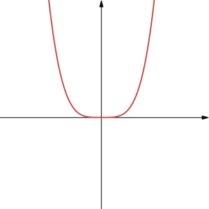
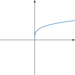
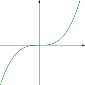
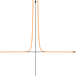
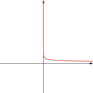
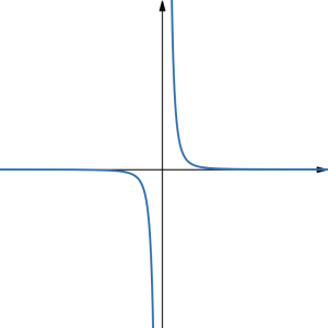
Here are some general shapes of graphs of power functions when the exponent is a non-zero whole number or a reciprocal of a non-zero whole number, based on whether the exponent is an even or and odd whole number:
 |
 |
 |
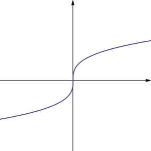 |
| [latex]y=x^{\text{even}}[/latex] | [latex]y=x^{1/(\text{even})}=\sqrt[\text{even}]{x}[/latex] | [latex]y=x^{\text{odd}}[/latex] | [latex]y=x^{1/(\text{odd})}=\sqrt[\text{odd}]{x}[/latex] |
 |
 |
 |
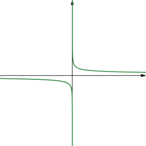 |
| [latex]y=x^{-(\text{even})}[/latex] | [latex]y=x^{-1/(\text{even})}=\frac{1}{\sqrt[\text{even}]{x}}[/latex] | [latex]y=x^{-(\text{odd})}[/latex] | [latex]y=x^{-1/(\text{odd})}=\frac{1}{\sqrt[\text{odd}]{x}}[/latex] |
A constant multiple of a power function is basically that: a constant value multiplied by a power function. As a result, it is a vertical stretch or compression of the underlying power function.
Some examples include: [latex]-4x,\ 1.2x^2,\ 6p^5,\ 0.03m^{-7},\ \frac{17}{21}x^{0.671}[/latex], etc.
It is important to learn this terminology, i.e., the definition of and the symbols used with the term power function and constant multiple of a (power) function because, when we get to derivatives and integrals, our ability to identify and apply appropriate differentiation rules will depend on our ability to recognize and name these types of functions.
When dealing with power functions, sometimes we use the term "power" to speak about the exponent or we use the ordinal version of the exponent. For example, to describe [latex]x^5[/latex] we may say:
"[latex]x[/latex] raised to the exponent of five"
"[latex]x[/latex] to the power of five"
"[latex]x[/latex] (raised) to the fifth"
We should never read this as "[latex]x[/latex] five"!
Note that multiplication is implied between the constant and the power function even if the multiplication symbol is omitted, such as in [latex]2x^5[/latex]. In particular, this should be read as "two times [latex]x[/latex] to the power of five" or "two times [latex]x[/latex] to the fifth" and, although it could be read as "two [latex]x[/latex] to the fifth", it should never be read as "two [latex]x[/latex] five".
Note also that, when writing power functions in a single line such as on calculators or on a computer, the symbol [latex]\hat{}[/latex] is used to denote the exponent and the symbols [latex]\times[/latex] and [latex]*[/latex] are used for multiplication (on the calculator and the computer, respectively). For example, we would write [latex]2\times x\hat{}5[/latex] on a calculator or [latex]2* x\hat{}5[/latex] in a computer code to represent [latex]2x^5[/latex]. In this case, if the exponent has multiple digits, we must mark this using parentheses, as in [latex]2\times x\hat{}(85)[/latex] or [latex]2* x\hat{}(85)[/latex] to represent [latex]2x^{85}[/latex]. This is one of the many reasons we should verbalize the operations when reading mathematical expressions even if the operation symbols in those expressions are omitted based on some convention.
Polynomial functions
A polynomial function is a version of stepping up from a power function. It is the fundamental building block of algebraic functions. You are likely to be familiar with the special cases of polynomial functions, such as the constant function, the linear function, and the quadratic function.
A polynomial function is a sum of constant multiples of power functions where the exponents in the power functions involved are non-negative integers. In particular, a polynomial function is the result of adding up a bunch of functions of the form [latex]ax^k[/latex] where [latex]a[/latex] is some constant value, [latex]x[/latex] is the variable, and [latex]k[/latex] is a whole number that is not negative (so, for example, exponents cannot be fractions or negative numbers).
Terminology of Polynomial Functions
A polynomial is a function that can be written as
[latex]f(x)=a_0+a_1 x+a_2 x^2+\dots+a_n x^n[/latex]
In a polynomial, the exponents on the variables can only be non-negative integers.
Since a polynomial function is defined only through addition and multiplication, which are defined for all real numbers, a polynomial function is defined on all real numbers, i.e., its domain is [latex]\mathbb{R}[/latex], or [latex](-\infty,\infty)[/latex].
Each of the [latex]a_i[/latex] constants are called coefficients and can be positive, negative, or zero, and be whole numbers, decimals, fractions or irrational numbers, i.e., they can be any real number.
A term of the polynomial is any one piece of the sum, that is any [latex]a_i x^i[/latex]. Each individual term is a constant multiple of a power function.
The degree of the polynomial is the highest exponent value on the variable that occurs in the polynomial.
The leading term is the term containing the highest exponent on the variable.
The leading coefficient is the coefficient of the leading term.
Because of the definition of the “leading” term, we often rearrange polynomials into so called standard form, where the exponents are descending:
[latex]f(x)=a_n x^n+a_{n-1}x^{n-1}+\dots +a_2 x^2+a_1 x+a_0[/latex]
Example 1
Answer: The degree is 3, the highest power on [latex]x[/latex]. The leading term is the term containing that power, [latex]-4x^3[/latex]. The leading coefficient is the coefficient of that term, -4.
General behaviour of polynomial functions
First of all, the domain of any polynomial function is the set of all real numbers, or [latex](-\infty, \infty)[/latex]. The range of a polynomial function will depend on its degree and on its leading coefficient. In particular, if the polynomial is of odd degree, its range will be all real numbers. If the polynomial is of even degree, then the range will be bounded by either a minimum (when the leading coefficient is positive) or by a maximum( when the leading coefficient is negative). This will become clearer through the discussion below.
In general, when studying a relationship between two quantities where one depends on another, we are interested both in what happens at specific points in this relationship (the specific input - output combinations) and also what happens generally, in terms of trends. More specifically, we are interested in what happens to the output values as we change the input values, most commonly as we increase the values of the input. We typically want to know when the output value is increasing and when it is decreasing, or perhaps remaining constant, in relation to an increase in the input value. We also want to know towards which what value the output is increasing or decreasing. The mathematical tools we use to make these determinations often boil down to the use of calculus tools, such as determining and analyzing the limit or the derivative of the function in relation to some given input. We will be discussing these tools in the sections to come. However, as in the case of power functions, there are some well known trends we can discern about polynomial functions, simply by looking at the leading term of the polynomial and analyzing the leading coefficient and the exponent, or the degree of the polynomial.
In particular, if we are considering a polynomial function of the form
[latex]f(x)=a_n x^n+a_{n-1}x^{n-1}+\dots +a_2 x^2+a_1 x+a_0[/latex]
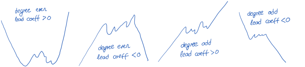
then the leading term is [latex]a_n x^n[/latex] and so the leading coefficient is [latex]a_n[/latex] and the degree of this polynomial is [latex]n[/latex]. Given this information, we can conclude the following, also illustrated in a drawing below, simply by considering whether the degree is an even or an odd number and whether the leading coefficient is a positive or a negative number:
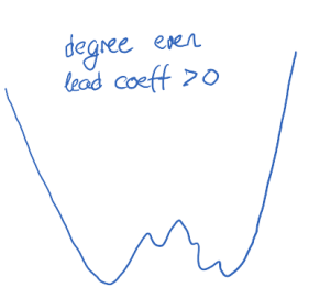
if [latex]n[/latex] is even and [latex]a_n x^n[/latex] is positive, [latex]f(x)[/latex] will get arbitrarily large or, as we say, will approach positive infinity (denoted by [latex]\infty[/latex]) as the input values get arbitrarily large in either the positive or the negative direction, graphically creating a "cup-like" shape with possibly some "bumps" at the bottom.
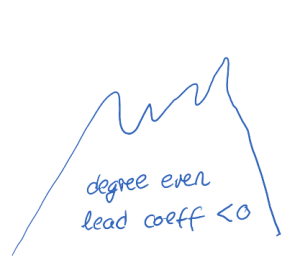
if [latex]n[/latex] is even and [latex]a_n x^n[/latex] is negative, [latex]f(x)[/latex] will approach negative infinity (denoted by [latex]-\infty[/latex]) as the input values get arbitrarily large in either the positive or the negative direction, graphically creating an inverted "cup-like" shape with possibly some "bumps" at the top.
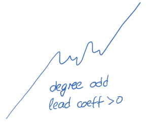
if [latex]n[/latex] is odd and [latex]a_n x^n[/latex] is positive, [latex]f(x)[/latex] will approach positive infinity as the input values approach positive infinity, and will approach negative infinity as the input values approach negative infinity, graphically creating an "upward mountain-like" shape with possibly some "bumps" in the middle.
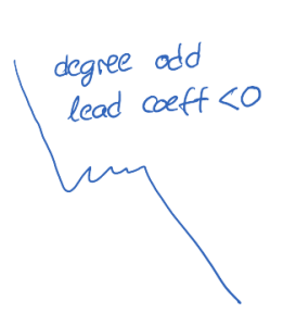
if [latex]n[/latex] is even and [latex]a_n x^n[/latex] is negative, [latex]f(x)[/latex] will approach negative infinity as the input values approach positive infinity, and will approach positive infinity as the input values approach negative infinity, graphically creating a "downward mountain-like" shape with possibly some "bumps" in the middle.
Granted, the description of the general trends provided above is not very technical in nature and so it is not quite precise. Later on in the course we will introduce more formal and thus more precise ways of speaking about the trends, however, for now, it is going to be helpful to us to be able to think about them in more general terms.
Example 2
Sketch the rough shape of the graph of each of the following polynomials in a way that it shows the general trends of the function and justify your drawing, then compare your sketch to the actual graph using a graphing tool of your choice.
a) [latex]f(x)=-7x^4+3x+1[/latex]
b) [latex]g(x)=7x^4+3x+1[/latex]
c) [latex]h(x)=7x^3+3x+1[/latex]
d) [latex]k(x)=-7x^4+3x+1[/latex]
Answer: For the general shape of a polynomial we need to identify the degree and the leading coefficient of the polynomial and determine whether they are even/odd and positive/negative, respectively. We then use that information to determine whether the shape is "cup-like" or "mountain-like", and whether it is oriented up(ward) or down(ward).
a) [latex]f(x)=-7x^4+3x+1\Rightarrow[/latex] degree is 4, which is even, and the lead coefficient is -7, or negative.
b) [latex]g(x)=7x^4+3x+1\Rightarrow[/latex] degree is 4, which is even, and the lead coefficient is 7, or positive.
c) [latex]h(x)=7x^3+3x+1\Rightarrow[/latex] degree is 3, which is odd, and the lead coefficient is 7, or positive.
d) [latex]k(x)=-7x^4+3x+1\Rightarrow[/latex] degree is 3, which is odd, and the lead coefficient is -7, or negative.
Therefore, the rough shape of each function is
 |
 |
 |
 |
| [latex]f(x)[/latex] | [latex]g(x)[/latex] | [latex]h(x)[/latex] | [latex]k(x)[/latex] |
The actual graphs can be visualized using the Desmos graphing tool: https://www.desmos.com/calculator/whxbfoejhw
Linear Functions
A linear function is a special case of a polynomial, where the degree of the polynomial is 1. As such, the general form of a linear function [latex]f(x)[/latex] is [latex]f(x)=a_1x+a_0[/latex] where [latex]a_0[/latex] and [latex]a_1[/latex] are real numbers and [latex]a_1\neq 0[/latex].
A linear function is a type of function that arises commonly in the every-day world and is also often used to model data relationships.
Characteristics of linear functions
A linear function is a function whose values change at a constant rate. Specifically, a function is linear if the change in output with respect to the corresponding change in input remains constant. Since a linear function is a polynomial, it is defined on all real numbers, i.e., its domain is [latex]\mathbb{R}[/latex], or [latex](-\infty,\infty)[/latex].
In tabular representation, the same increase (or decrease) in the input value will result in a constant change in the output value.
In formulaic representation we can represent a linear function as [latex]f(x)=mx+b[/latex], where the values of [latex]m[/latex] and [latex]b[/latex] represent the following:
[latex]m=\frac{\text{change in output}}{\text{change in input}}=\dfrac{\Delta \text{output}}{\Delta \text{input}}=\frac{\text{output}_2-\text{output}_1}{\text{input}_2-\text{input}_2}=\frac{f(x_2)-f(x_1)}{x_2-x_1}[/latex]
[latex]b=\text{the output value when the input value is 0}=f(0)[/latex]
Note that the symbol [latex]\Delta[/latex], read as "delta", is the upper case Greek letter for d, representing difference, or change.
The graph of a linear function produces a straight line. The slope of that line is equal to
[latex]m=\frac{\text{change in output}}{\text{change in input}}[/latex]
and the vertical intercept of that line is equal to
[latex]b=\text{the output value when the input value is 0}[/latex].
The rate of change value determines if the function is increasing, decreasing or constant:
- If [latex]m\gt 0[/latex], [latex]f(x)=mx+b[/latex] is an increasing function.
- If [latex]m\lt 0[/latex], [latex]f(x)=mx+b[/latex] is a decreasing function.
- If [latex]m=0[/latex], the function [latex]f(x)=0x+b=b[/latex] is just a horizontal line passing through the point [latex](0, b)[/latex], neither increasing nor decreasing.
Concept Check
Mathmatize: Linear or not?
Example 3
The population of a city increased from 23,400 to 27,800 between 2002 and 2006. Assuming that the population grew at a constant rate, find the rate of change of the population during this time span and interpret the result.
Answer: rate of change? interpretation?
Rate of change: Since the assumption is that the population is growing at a constant rate, this is a linear relationship and the rate of change will relate the change in output to the change in input. In this relationship, the output is the size of the population and the input is the year. Therefore,
[latex]\begin{align*} \text{rate of change}&=\dfrac{\text{change in output}}{\text{change in input}}=\dfrac{\text{change in population size}}{\text{change in # of years}}\\ &=\dfrac{27800-23400}{2006-2002}=\dfrac{4400}{4}=1100\end{align*}[/latex]
This means that between 2002 and 2006 the population was increasing by 1100 people per year.
(Note that we knew the population was increasing, so we would expect our value for the rate of change to be positive. This is a quick way to check to see if your value for the rate of change is reasonable.)
Visual demonstration
Follow the link below to see the effect on the graph of a linear function [latex]f(x)=mx+b[/latex] while changing the value of rate of change parameter [latex]m[/latex] and the initial value [latex]b[/latex].
Concept Check
MathMatize: Reading and interpreting linear functions
Quadratic functions
Quadratic functions, also called quadratics, are a special case of a polynomial function, where the degree of the polynomial is 2.
Every function that can be written in the form [latex]f(x)=ax^2+bx+c[/latex] for some real numbers [latex]a, b[/latex] and [latex]c[/latex] where [latex]a\neq 0[/latex] is a quadratic function and every quadratic function can be written in this form.
Characteristics of quadratic functions
Every quadratic function can be represented through its standard form:
[latex]f(x)=ax^2+bx+c[/latex]
where [latex]a, b[/latex] and [latex]c[/latex] are real numbers and [latex]a\neq 0[/latex]. The value [latex]a[/latex] is called the leading coefficient and [latex]c[/latex] is the constant term. Since a quadratic function is a polynomial, it is defined on all real numbers, i.e., its domain is [latex]\mathbb{R}[/latex], or [latex](-\infty,\infty)[/latex].
Some quadratic functions can also be represented through the factored form:
[latex]f(x)=a(x-x_1)(x-x_2)[/latex]
where [latex]a, x_1[/latex] and [latex]x_2[/latex] are real numbers and [latex]a\neq 0[/latex]. The values [latex]x_1[/latex] and [latex]x_2[/latex] represent the zeros of the function, i.e., the input values making the output value of the function 0. They are determined using the quadratic formula:
[latex]x_{1,2}=\frac{-b\pm\sqrt{b^2-4ac}}{2a}[/latex]
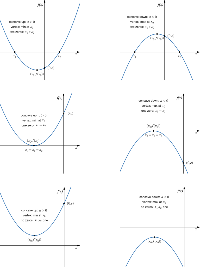
A graph of a quadratic function is a parabola, a cup-like shape that opens up (concaves up) if the leading coefficient [latex]a[/latex] is a positive number and opens down (concaves down) if the leading coefficient [latex]a[/latex] is a negative number. The lowest or the highest point of the parabola, depending on the concavity, is called a vertex and its coordinates are:
[latex](x_0,f(x_0))=\left(-\frac{b}{2a},f\left(-\frac{b}{2a}\right)\right)[/latex]
The vertical intercept of a graph of a quadratic function is the value of the constant term, i.e., it is the point [latex](0,f(0))=(0,c)[/latex]. The horizontal intercepts, if any, are the zeros of the function, i.e., [latex](x_1,0)[/latex] and [latex](x_2,0)[/latex] where [latex]x_1[/latex] and [latex]x_2[/latex] can be determined using the quadratic formula.
The most commonly used form of a quadratic equation is the standard form but either one, standard or factored form, can be useful in different contexts because they provide direct information about the behaviour of the quadratic function:
- The standard form provides information about the orientation of the graph ([latex]a[/latex]) and its vertical intercept ([latex]c[/latex]).
- The factored form gives us the information about the orientation of the graph ([latex]a[/latex]) and where the graph intercepts the horizontal axis ([latex]x_1[/latex] and [latex]x_2[/latex]).
Note that the graph of every quadratic function will have a vertex but not every quadratic function will have zeros. This is because, to calculate the zeros we use the quadratic formula, which includes a calculation of a square root, and a square root can only be calculated on non-negative numbers - a square root of a negative number does not exist (in real numbers). In general, a quadratic function will have two, one or no zeros, depending on the value of its discriminant [latex]D=b^2-4ac[/latex]:
If [latex]D=b^2-4ac\gt 0[/latex] then the function has two zeros.
If [latex]D=b^2-4ac=0[/latex] then the function has one zero.
If [latex]D=b^2-4ac\lt 0[/latex] then the function has no zeros.
There are six types of graphs arising from quadratic equations, determined by the orientation of the parabola and the location of the vertex, which together determine how how many zeros the function has (two, one or none):
Example 4
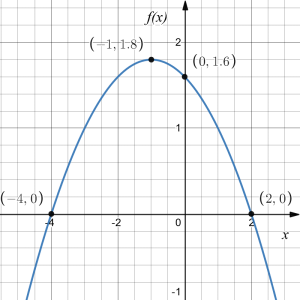
Determine the orientation, the vertical intercept, the coordinates of the vertex and the horizontal intercepts of the quadratic function, and sketch its graph if its standard and factored form are
[latex]\begin{align*} f(x)&=-\frac{1}{5}x^2-\frac{2}{5}x+\frac{8}{5}&\text{standard form} \\ &=-\frac{1}{5}(x-2)(x+4)&\text{factored form} \end{align*}[/latex]
Answer: From standard form [latex]f(x)=ax^2+bx+c[/latex] we can see that the parabola is oriented downwards because the leading coefficient, i.e., the coefficient of [latex]x^2[/latex], is [latex]-\frac{1}{5}[/latex], which is a negative number. Also, since the constant term in the standard form, i.e., the term with no variable, is [latex]\frac{8}{5}[/latex], the vertical intercept is at the point [latex]\left(0,1.6\right)[/latex].
Finally, the factored form [latex]f(x)=a(x-x_1)(x-x_2)[/latex] tells us that [latex]f(x)=0[/latex] only if [latex]a(x-x_1)(x-x_2)=0[/latex]. Since [latex]a[/latex] is a non-zero number and the only way we can get the value zero from multiplication is if one of the factors being multiplied is zero, we have that the only solutions to that equation are [latex]x_1=2[/latex] and [latex]x_2=-4[/latex]. Therefore, the zeros of the function are 2 and -4 and so the horizontal intercepts are at points [latex](2,0)[/latex] and [latex](-4,0)[/latex].
It is very important to note that the quadratic formula solves the equation [latex]ax^2+bx+c=0[/latex], i.e., determines the values of [latex]x[/latex] that satisfy [latex]f(x)=0[/latex]. There are other methods for solving a quadratic equation that can be used in some special cases, but the quadratic formula will always work if there are solutions. Recall that, if a quadratic expression can be factored, it can always be factored as follows:
[latex]f(x)=a(x-x_1)(x-x_2)[/latex] where [latex]x_{1,2}=\dfrac{-b\pm \sqrt{b^2-4ac}}{2a}[/latex]
Note that this is the abbreviated version of writing [latex]x_{1}=\frac{-b+ \sqrt{b^2-4ac}}{2a}[/latex] and [latex]x_{2}=\frac{-b- \sqrt{b^2-4ac}}{2a}[/latex]. Also note that there are no possibilities for [latex]x_1[/latex] and [latex]x_2[/latex] if the discriminant, [latex]b^2-4ac[/latex], is a negative number.
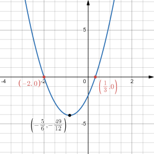
Example 4
Determine the vertex and the vertical and horizontal intercepts of the quadratic [latex]f(x)=3x^2+5x-2[/latex], graph the function, and write it in factored form.
Answer:
vertex: We can use the standard form in which [latex]f(x)[/latex] is written and so the vertex is located at [latex](x_0,f(x_0))[/latex] where
[latex]x_0=-\dfrac{b}{2a}=-\dfrac{5}{2\cdot(3)}=-\dfrac{5}{6}[/latex]
Since
[latex]f\left(-\dfrac{5}{6}\right)=3\left(-\dfrac{5}{6}\right)^2+5\left(-\dfrac{5}{6}\right)-2=-\dfrac{49}{12}[/latex]
the vertex is located at the point [latex]\left(-\frac{5}{6},-\frac{49}{12}\right)[/latex].
vertical intercept: The vertical intercept occurs when the input value is zero: [latex]f(0)=3(0)^2+5(0)-2=-2[/latex] Equivalently, we can use the standard form of [latex]f(x)[/latex] and the fact that the vertical intercept occurs at [latex](0,c)[/latex], and so the vertical intercept is at (0,-2).
horizontal intercepts: The horizontal intercepts occur when the output is zero, i.e., [latex]f(x)=0[/latex]: [latex]0=3x^2+5x-2.[/latex] To solve this equation we can use the quadratic formula:
[latex]\begin{align*} x_{1,2}&=\frac{-b\pm \sqrt{b^2-4ac}}{2a}\\ & =\frac{-5\pm \sqrt{5^2-4\cdot 3\cdot (-2)}}{2\cdot 3}\\ &=\frac{-5\pm 7}{6}\\ \Rightarrow&x_1=\frac{-5+ 7}{6}=\frac{1}{3}\\ &x_2=\frac{-5-7}{6}=-2 \end{align*}[/latex]
So the horizontal intercepts are at [latex]\left(\frac{1}{3},0\right)[/latex] and [latex](-2,0)[/latex].
Using all of the information above, we can now sketch the graph of this function:
factored form: Using the fact that [latex]x_1=\frac{1}{3}[/latex] and [latex]x_2=-2[/latex] are the zeros of the quadratic function [latex]f(x)[/latex], we can rewrite [latex]f(x)[/latex] as
[latex]f(x)=a(x-x_1)(x-x_2)=5\left(x-\frac{1}{3}\right)(x+2)[/latex]
You can verify all of the above by using a graphing calculator, say Desmos: link, however you must be able to justify all characteristics algebraically as above.
Rational Functions
Rational functions are the ratios, or fractions, of polynomials.
Characteristics of rational functions
A rational function is a function that can be written as the ratio of two polynomials, [latex]P(x)[/latex] and [latex]Q(x)[/latex]:
[latex]f(x)=\frac{P(x)}{Q(x)}=\frac{a_p x^p+a_{p-1} x^{p-1}+\ldots a_2 x^2 + a_1 x+a_0 }{b_q x^q+b_{q-1} x^{q-1}+\ldots b_2 x^2 + b_1 x+b_0 }[/latex]
Since a rational function represents division of two values that can be calculated for all real numbers (because they are represented through polynomials), the value of a rational function cannot be calculated only if the polynomial in the denominator is equal to zero. Therefore, the domain of a rational function is all real numbers except the zeros of the denominator polynomial, i.e., its domain is [latex]\{x\in\mathbb{R}|Q(x)\neq 0\}[/latex].
Zeros of a rational function, i.e., the values for which [latex]f(x)=\frac{P(x)}{Q(x)}=0[/latex] are the values of [latex]x[/latex] in the domain of [latex]f(x)[/latex] for which the numerator polynomial [latex]P(x)[/latex] is equal to zero.
Graphically, the zeros of a rational function will give the horizontal intercepts and the vertical intercept will occur at [latex]f(0)=\frac{a_0}{b_0}[/latex].
Rational functions can exhibit the so called asymptotic behaviour as the values of the input variable increase towards [latex]\infty[/latex] and as they decrease [latex]-\infty[/latex], but this is not always the case. We say that the rational function has a horizontal asymptote if the values of [latex]f(x)[/latex] approach a specific value as [latex]x[/latex] approaches [latex]\infty[/latex] or [latex]-\infty[/latex].
The graph of a rational function will also have a hole or a vertical asymptotes at values on the horizontal axis that are excluded from the function's domain. (We will learn how to identify them in an upcoming section where we discuss limits of a function.)
We will discuss the behaviour of rational functions in greater details later on when we discuss the limit of a function at a point and at infinities. Here are some examples of rational functions and their graphs:
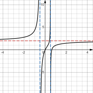 |
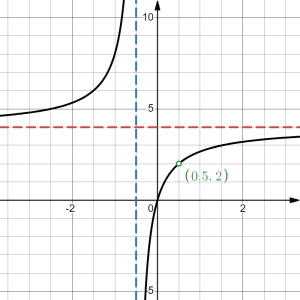 |
| [latex]A\left(x\right)=\frac{8x^{2}-5x}{4x^{2}-1}[/latex] | [latex]B\left(x\right)=\frac{16x^{2}-8x}{4x^{2}-1}[/latex] |
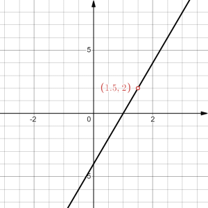 |
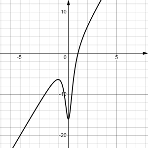 |
| [latex]C\left(x\right)=\frac{16x^{2}-24x+8}{4x-2}[/latex] | [latex]D\left(x\right)=\frac{16\left(x^{3}-1\right)}{4x^{2}+1}[/latex] |
Exercises
Work on the following exercises. Discuss your solutions with your peers and/or course instructor.
IC4NITS Exercises 1.4 - Algebraic Functions
