1.3 Operations on Functions
1.3 Operations on Functions
In this section we will discuss, in a formal way and through examples, the following concepts: operations on functions such as addition, subtraction, multiplication, division, and composition, as well as transformations as special cases of compositions. We will also learn to analyze a function through a lens of operations on multiple functions using analysis of the algebraic operations and the order of those operations involved in the given function. The latter will be extremely important when we get to derivatives and are determining which rules to apply to calculate the derivative of a function.
____________________________
Operations on functions
Since functions represent relationships through rules applied to an input value to produce an output value, we can sometimes combine the rules given to create new outputs from the same input.
For example, we may start with two functions: one that describes how many front-line technician hours are required to complete a particular type of task, and another that describes how many office support hours are required, given a type of task. We can then create a new function from those two by combining the rules through addition to describe the total number of hours required given a specific type of task.
Another example may be where a business analyst has created a function to model the number of households within some region at a given time and has also created a model to describe the probability that a household in that region will purchase the service provided by the business at a given time. These two models can then be used to predict the overall number of households purchasing the service, a valuable information for business planning. The new model will be the product of the overall number of households at the given time and the probability that a household purchases the service at that time. In other words, the function representing the new model will be the product of the two original functions.
Consider one more example before we formalize the language of operations on functions: Computing the latency of a network (the time from the moment a computer—usually a server—receives a request to the time it returns a response) depends on different factors, including amount of data that needs to be processed, the computing architecture capacity, and the algorithm complexity. In turn, the amount of data that needs to be processed could be considered in terms of the number of users, so therefore the compute latency depends on the number of users through the relationship between each and the amount of data processed. In other words, if we can use a function to model the amount of data to be processed given a number of users, and if we can use another function to model the compute latency given the amount of data to be processed, we can create a new function that will describe the compute latency as the output given the number of users as an input through the so called composition of the two original functions. In the world of coding, this new function will often be called a nested function.
In general, we can combine functions in different ways through operations of:
Addition: [latex](𝑓+𝑔)(𝑥)= 𝑓(𝑥)+𝑔(𝑥)[/latex]
Subtraction: [latex](𝑓−𝑔)(𝑥)= 𝑓(𝑥)−𝑔(𝑥)[/latex]
Multiplication: [latex](𝑓\cdot 𝑔)(𝑥)= 𝑓(𝑥)\cdot 𝑔(𝑥)[/latex]
Division: [latex]\left(\dfrac{f}{g}\right)(x)=\dfrac{f(x)}{g(x}; \ \ \ \ \ \ \ g(x)\neq 0[/latex]
Composition: [latex](f\circ g)(x)=f(g(x))[/latex]
The first four operations should not be surprising or complex to do, but one, as always, must be careful. Here is an example of all five operations in action:
Suppose
[latex]f(x)=x^2-3x+4[/latex] and [latex]g(x)=x-50[/latex]
Then,
[latex](f+g)(x)=f(x)+g(x)=x^2-3x+4+x-50=x^2-2x-46[/latex]
[latex]\begin{align*}(f-g)(x)&=f(x)-g(x)=x^2-3x+4-(x-50)\\ &=x^2-3x+4-x+50=x^2-4x+54\end{align*}[/latex]
[latex]\begin{align*}(f\cdot g)(x)&=f(x)\cdot g(x)=(x^2-3x+4)\cdot(x-50)\\ &=x^3-50x^2-3x^2+150x+4x-200\\ &=x^3-53x^2+154x-200\end{align*}[/latex]
[latex]\left(\dfrac{f}{g}\right)(x)=\dfrac{f(x)}{g(x)}=\begin{cases}\frac{x^2-3x+4}{x-50}& \text{if } x\neq 50\\ \text{undefined}&\text{ if } x=50\end{cases}[/latex]
[latex]\begin{align*}\left(f\circ g\right)(x)&=f(g(x))=f(x-50)\\ &=(x-50)^2-3(x-50)+4\\ &=x^2-100x+2500-3x+150+4\\ &=x^2-103x+2654 \end{align*}[/latex]
Note the importance of using brackets when appropriate. Some of the most common mistakes students make are in subtraction, multiplication and composition by forgetting to add brackets appropriately or by not removing them appropriately through algebraic operations on the expressions involved.
Composition of Functions
The last operation listed above is the composition of functions. It is used when one function is applied on the result of another function. We discussed already one example when it might come into play, such as in the relationships between compute latency, amount of processed data, and the number of users. Here is another example:
Suppose we wanted to calculate how much it costs to heat a house on a particular day of the year. The cost to heat a house will depend on the average daily temperature, and the average daily temperature depends on the particular day of the year.
Notice how we have just defined two relationships: The cost depends on the temperature and the temperature depends on the day. Using descriptive variables, we can use the function notation for these two functions:
The first function, [latex]C(T)[/latex], gives the cost [latex]C[/latex] of heating a house when the average daily temperature is [latex]T[/latex] degrees Celsius, and the second, [latex]T(d)[/latex], gives the average daily temperature of a particular city on day [latex]d[/latex] of the year. If we wanted to determine the cost of heating the house on the fifth day of the year, we could do this by linking our two functions together, an idea called composition of functions. Using the function [latex]T(d)[/latex], we could evaluate [latex]T(5)[/latex] to determine the average daily temperature on the fifth day of the year. We could then use that temperature as the input to the [latex]C(T)[/latex] function to find the cost to heat the house on the fifth day of the year: [latex]C(T(5))[/latex].
Function composition vocabulary
When the output of one function is used as the input of another, we call the entire operation a composition of functions.
The composition operation uses the composition operator: [latex]\circ[/latex]
Using the composition operator, [latex](f\circ g)(x)[/latex] is read “f of g of x” or “f composed with g at x”, and it represents [latex]f(g(x))[/latex]. We refer to [latex]g[/latex] as the inner function and to [latex]f[/latex] as the outer function.
Note that the range of the inner function must be within the domain of the outer function for the composition to be defined on the domain of the inner function.
We can also have more than two functions involved in a composition. For example,
[latex](f\circ g\circ h\circ k\circ l\circ m)(x)=f(g(h(k(l(m(x))))))[/latex]
Example 1
Suppose [latex]c(s)[/latex] gives the number of calories burned doing [latex]s[/latex] sit-ups, and [latex]s(t)[/latex] gives the number of sit-ups a person can do in [latex]t[/latex] minutes. Interpret [latex]c(s(3))[/latex].
Answer:
When we are asked to interpret, we are being asked to explain the meaning of the expression in words. The inside expression in the composition is [latex]s(3)[/latex]. Since the input to the [latex]s[/latex] function is time, the 3 is representing 3 minutes, and [latex]s(3)[/latex] is the number of sit-ups that can be done in 3 minutes. Taking this output and using it as the input to the [latex]c(s)[/latex] function will give us the calories that can be burned by the number of sit-ups that can be done in 3 minutes.
Composition of functions using tables and graphs
When working with functions given as tables and graphs, we can look up values for the functions using a provided data table or graph. We start evaluation from the provided input, and first evaluate the inside function. We can then use the output of the inside function as the input to the outside function. To remember this, always work from the inside out.
Example 2
Using the graphs below, evaluate [latex](f\circ g)(1)[/latex].
 |
 |
| [latex]g(x)[/latex] | [latex]f(x)[/latex] |
Answer: To evaluate [latex](f\circ g)(1)[/latex], we start with the inside evaluation. We evaluate [latex]g(1)[/latex] using the graph of the [latex]g(x)[/latex] function, finding the input of 1 on the horizontal axis and finding the output value of the graph at that input. Here, [latex]g(1)=3[/latex]. Using this value as the input to the [latex]f[/latex] function, [latex]f(g(1))=f(3)[/latex]. We can then evaluate this by looking to the graph of the [latex]f(x)[/latex] function, finding the input of 3 on the horizontal axis, and reading the output value of the graph at this input. Here, [latex]f(3)=6[/latex], so [latex]f(g(1))=6[/latex]. Mathematically, we write this process as follows:[latex](f\circ g)(1)=f(g(1))=f(3)=6[/latex]
Compositions using formulas
When evaluating a composition of functions where we have either created or been given formulas, the concept of working from the inside out remains the same. First we evaluate the inside function using the input value provided, then use the resulting output as the input to the outside function.
Example 3
Given [latex]f(x)=x^2-x[/latex] and [latex]h(x)=3x+2[/latex], find [latex](f\circ h)(x)[/latex] and evaluate [latex](f\circ h)(1)[/latex].
Answer:
[latex]\begin{align*} (f\circ h)(x)&=f(h(x))=f(3x+2)=(3x+2)^2-(3x+2)\\ & =9x^2+12x+4-3x-2\\ &=9x^2+9x+2 \end{align*}[/latex]
From this it follows that
[latex](f\circ h)(1)=9(1)^2+9(1)+2=20[/latex]
Note that, unlike addition and multiplication, which are commutative (i.e., the order does not matter), composition is, like subtraction and division, not commutative. In other words, just like the order of values matters in subtraction and division, the order will also matter in composition, i.e., in general we'll have that [latex](f\circ g)(x)\neq (g\circ f)(x)[/latex].
Example 4
Let [latex]f(x)=x^2[/latex] and [latex]g(x)=\dfrac{1}{x}-2x[/latex]. Find [latex](f\circ g)(x)[/latex] and [latex](g\circ f)(x)[/latex].
Answer:
To find [latex]f(g(x))[/latex], note that [latex]f[/latex] is applied to [latex]g[/latex] and so [latex]g[/latex] is the inside function and [latex]f[/latex] is the outside function. So we have:
[latex](f\circ g)(x)=f(g(x))=f\left(\dfrac{1}{x}-2x\right) =\left(\dfrac{1}{x}-2x\right)^2[/latex]
Likewise, to find [latex]g(f(x))[/latex], we evaluate the inside, which is [latex]f(x)[/latex], and then we evaluate [latex]g(x)[/latex] using [latex]f(x)[/latex] as the input:
[latex](g\circ f)(x)=g(f(x))=g(x^2)=\dfrac{1}{x^2}-2x^2[/latex]
As expected, note that the expressions for [latex](f\circ g)(x)[/latex] and [latex](g\circ f)(x)[/latex] in the above example were different. This is true in general. The order matters in compositions of functions and, except in very specific cases, the resulting function is different if the inside and the outside functions are reversed. The ability to distinguish which function is an inner function and which one is an outer function will be of high importance when we get to derivatives (and integrals) and are using the derivative rule that applies to compositions of functions.
Example 5
A city manager determines that the tax revenue, [latex]R[/latex], in millions of dollars collected on a population of [latex]p[/latex] thousand people can be modeled by the function [latex]R(p)=0.03p+\sqrt{p}[/latex] and that the city’s population, in thousands, is predicted to follow the formula [latex]p(t)=60+2t+0.3t^2[/latex], where [latex]t[/latex] is measured in years after 2010. Find the formula for the tax revenue as a function of the year.
Answer:
Since we want tax revenue as a function of the year, we want year to be our initial input, and revenue to be our final output. To find revenue, we will first have to predict the city population, and then use that result as the input to the tax function. So we need to find [latex](R\circ p)(t)).[/latex] Evaluating this,
[latex]\begin{align*} (R\circ p)(t))&=R(p(t)) = R(60+2t+0.3t^2)\\ & = 0.03(60+2t+0.3t^2)+\sqrt{60+2t+0.3t^2} \end{align*}[/latex]
This composition gives us a single formula which can be used to predict the tax revenue during a given year, without needing to find the intermediary population value. For example, to predict the tax revenue in 2017, when [latex]t = 7[/latex] (because [latex]t[/latex] is measured in years after 2010),
[latex]\begin{align*} (R\circ p)(7))&=R(p(7)) \\ &= 0.03\left(60+2(7)+0.3\left(7^2\right)\right)+\sqrt{60+2(7)+0.3\left(7^2\right)}\\ &\approx 12.079\text{ million dollars} \end{align*}[/latex]
Later in this course it will be necessary to know how to decompose a composite function, i.e. to write it as a composition of two or more simpler functions. The following example demonstrates the process.
Example 6
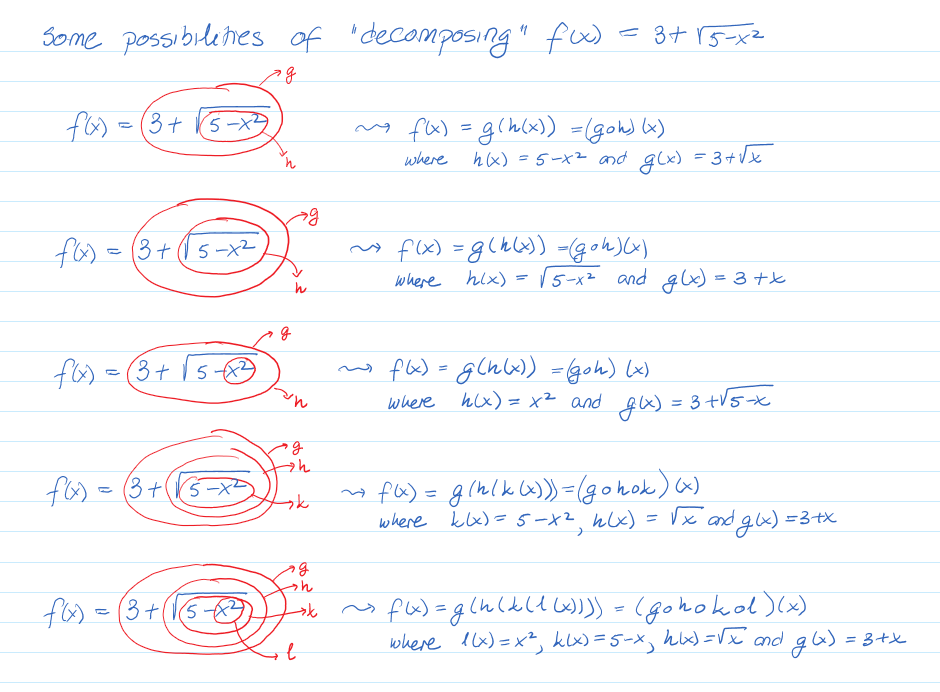
Write [latex]f(x)=3+\sqrt{5-x^2}[/latex] as a composition of functions.
Answer: We are looking for two functions, [latex]g[/latex] and [latex]h[/latex], so that [latex]f(x)=g(h(x))[/latex]. To do this, we look for a function inside a function in the formula for [latex]f(x)[/latex].
As one possibility, we note that the square root component cannot be calculated before [latex]5-x^2[/latex] is calculated. So that tells us that there are layers of functions and [latex]5-x^2[/latex] can be thought of as the inside function. Once [latex]5-x^2[/latex] is calculated, then one can take the square root of it and add 3 to get the final result. So this tells us that we can decompose the function [latex]f(x)[/latex] using [latex]h(x)=5-x^2[/latex] and [latex]g(x)=3+\sqrt{x}[/latex], where [latex]h[/latex] is the inner and [latex]g[/latex] is the outer function.
We can check our answer by recomposing the functions:
[latex](g\circ h)(x)=g(h(x))=g(5-x^2)=3+\sqrt{5-x^2}=f(x)[/latex]
Note that this is not the only solution to the problem. Another non-trivial decomposition would be [latex]h(x)=x^2[/latex], and [latex]g(x)=3+\sqrt{5-x}[/latex]. Verify.
Here are some more options:
Concept Check
Test your understanding of how to determine compositions of functions using their formulas.
MathMatize: Compositions of functions
Transformations of functions
One application of compositions of functions is transformations of functions. Transformations allow us to construct new functions from our basic types of functions. We will discuss the following transformations:
- vertical shift upwards or downwards
- horizontal shift left or right
- vertical stretch/compression
- horizontal stretch/compression
- reflection in the [latex]x[/latex] axis
- reflection in the [latex]y[/latex] axis
Here is the summary:
| Transformation | Original function | New function |
| Vertical shift upward by [latex]c[/latex] | [latex]f(x)\longrightarrow[/latex] | [latex]𝑔(𝑥)=𝑓(𝑥)+𝑐[/latex] |
| Vertical shift downward by [latex]c[/latex] | [latex]f(x)\longrightarrow[/latex] | [latex]𝑔(𝑥)=𝑓(𝑥)−𝑐[/latex] |
| Horizontal shift to the left by [latex]c[/latex] | [latex]f(x)\longrightarrow[/latex] | [latex]𝑔(𝑥)=𝑓(𝑥+𝑐)[/latex] |
| Horizontal shift to the right by [latex]c[/latex] | [latex]f(x)\longrightarrow[/latex] | [latex]𝑔(𝑥)=𝑓(𝑥−𝑐)[/latex] |
| Vertical stretch by a factor of [latex]c[/latex] | [latex]f(x)\longrightarrow[/latex] | [latex]𝑔(𝑥)=𝑐𝑓(𝑥)[/latex] |
| Vertical compression by a factor of [latex]c[/latex] | [latex]f(x)\longrightarrow[/latex] | [latex]𝑔(𝑥)=\frac{1}{𝑐}𝑓(𝑥)[/latex] |
| Horizontal stretch by a factor of [latex]c[/latex] | [latex]f(x)\longrightarrow[/latex] | [latex]𝑔(𝑥)=𝑓(\frac{1}{𝑐}𝑥)[/latex] |
| Horizontal compression by a factor of [latex]c[/latex] | [latex]f(x)\longrightarrow[/latex] | [latex]𝑔(𝑥)=𝑓(𝑐𝑥)[/latex] |
| Reflection in the [latex]x[/latex]-axis | [latex]f(x)\longrightarrow[/latex] | [latex]𝑔(𝑥)=−𝑓(𝑥)[/latex] |
| Reflection in the [latex]y[/latex]-axis | [latex]f(x)\longrightarrow[/latex] | [latex]𝑔(𝑥)=𝑓(−𝑥)[/latex] |
Let's look at each of them individually and discuss why the formulas provided above represent those transformations, and how we can build those formulas from understanding the transformation process.
Vertical shift
Given a function [latex]f(x)[/latex], if we define a new function [latex]g(x)[/latex] as [latex]g(x)=f(x)+k[/latex], where [latex]k[/latex] is a constant, then [latex]g(x)[/latex] is a vertical shift of the function [latex]f(x)[/latex], where all the output values have been increased by [latex]k[/latex].
If [latex]k[/latex] is positive, then the graph will shift up. If [latex]k[/latex] is negative, then the graph will shift down.
Conversely, if we wish to shift every point on the graph up (or down) by a certain constant value, effectively we are keeping the horizontal coordinates the same and changing the vertical coordinate by adding (or subtracting) the constant value. Since the horizontal coordinate represents the input of the function and the vertical coordinate represents the output of the function, the input will remain the same while the output value is increased (or decreased) by the constant.
For example, consider the function
[latex]f(x)=3-\sqrt{2x^2+1}[/latex]
Then shifting this function up by, say, [latex]5[/latex], would result in a new function
[latex]g(x)=f(x)+5=3-\sqrt{2x^2+1}+5=8-\sqrt{2x^2+1}[/latex]
and shifting [latex]f(x)[/latex] down by [latex]5[/latex] would result in yet another function
[latex]h(x)=f(x)-5=3-\sqrt{2x^2+1}-5=-2-\sqrt{2x^2+1}[/latex]
Visual demonstration:
Follow the link below and use the slider for the vertical shift parameter [latex]k[/latex] to see the effect of adding [latex]k[/latex] to the value of function [latex]f(x)[/latex]. In this demonstration we use the function [latex]f(x)=x^3[/latex] but you can change it to a function of your choice and vary the value of [latex]k[/latex] using the slider to explore this transformation in different settings.
Horizontal shift
Given a function [latex]f(x)[/latex], if we define a new function [latex]g(x)[/latex] as [latex]g(x)=f(x+k)[/latex], where [latex]k[/latex] is a constant, then [latex]g(x)[/latex] is a horizontal shift of the function [latex]f(x)[/latex], where all the input values have been increased by [latex]k[/latex].
If [latex]k[/latex] is positive, then the graph will shift left. If [latex]k[/latex] is negative, then the graph will shift right.
Conversely, if we wish to shift every point on the graph left (or right) by a certain constant value, effectively we are keeping the vertical coordinates (or the output) the same and changing the horizontal coordinate (or the input) by this constant value. The mathematics of this shift requires us to apply this constant counter-intuitively (a similar thing will occur with another horizontal transformation: horizontal stretch/compression): if we want to move to the left, we have to add the constant to the input variable, and if we want to move to the right, we have to subtract the constant from the input.
For example, consider the function
[latex]f(x)=3-\sqrt{2x^2+1}[/latex]
Then shifting this function left by, say, [latex]5[/latex], would result in a new function
[latex]\begin{align*}k(x)&=f(x+5)=3-\sqrt{2(x+5)^2+1}\\ &=3-\sqrt{2(x^2+10x+25)+1}\\ &=3-\sqrt{2x^2+20x+51}\end{align*}[/latex]
and shifting [latex]f(x)[/latex] right by [latex]5[/latex] would result in yet another function
[latex]\begin{align*}l(x)&=f(x-5)=3-\sqrt{2(x-5)^2+1}\\ &=3-\sqrt{2(x^2-10x+25)+1}\\ &=3-\sqrt{2x^2-20x+51}\end{align*}[/latex]
Visual demonstration:
Follow the link below and use the slider for the horizontal shift parameter [latex]k[/latex] to see the effect of adding [latex]k[/latex] to the value of [latex]x[/latex]. In this demonstration we use the function [latex]f(x)=x^3[/latex] but you can change it to a function of your choice and vary the value of [latex]k[/latex] using the slider to explore this transformation in different settings.
Example 7
Given [latex]f(x)=|x|[/latex], determine the transformations applied to [latex]f(x)[/latex] to result in [latex]h(x)=|x+1|-3[/latex] and sketch the graph of [latex]h(x)[/latex].
Answer: transformations? graph of new function?
Transformations: To determine which transformations were applied to arrive from[latex]f(x)[/latex] to [latex]h(x)[/latex] we effectively have to start with [latex]f(x)[/latex] and, step by step, analyze which operations are taking place, and in which order, to get from the formula of [latex]f(x)[/latex] to the formula of [latex]h(x)[/latex]:
| [latex]f(x)=|x|[/latex] | |
| [latex]\quad \big\downarrow[/latex] | |
| [latex]f_1(x)=|x+1|=f(x+1)[/latex] | [latex]\longleftarrow[/latex] shift [latex]f(x)[/latex] to the left by [latex]1[/latex], followed by |
| [latex]\quad \big\downarrow[/latex] | |
| [latex]f_2(x)=|x+1|+3=f_1(x)-3[/latex] | [latex]\longleftarrow[/latex] shift [latex]f_1(x)[/latex] down by [latex]3[/latex] |
| Therefore, | |
| [latex]h(x)=f_2(x)=f_1(x)-3=f(x+1)-3[/latex] | [latex]\longleftarrow[/latex] shift [latex]f(x)[/latex] to the left by [latex]1[/latex], then down by [latex]3[/latex] |
New graph: The function [latex]|x|[/latex] is our basic absolute value function. We know that this graph has a V shape, with the point at the origin. The graph of [latex]h[/latex] has transformed [latex]f[/latex] in two ways: shift [latex]f(x)[/latex] to the left by [latex]1[/latex], then down by [latex]3[/latex]. Transforming the graph from [latex]f(x)[/latex] to [latex]h(x)[/latex] gives:
| [latex]\to[/latex] | [latex]\to[/latex] | |||
| [latex]f(x)=|x|[/latex] | [latex]f_1(x)=|x+1|=f(x+1)[/latex] | [latex]f_2(x)=|x+1|+3=f_1(x)-3[/latex] |
Example 8
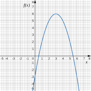
Determine the formula for the graph of [latex]f(x)[/latex] shown below as a transformation or a series of transformations of the square root function [latex]h(x)=\sqrt{x}[/latex].
![]()
![]() Answer:
Answer:
We start with the graph of the square root function, which is on the right.
To get a sense of what is happening to the points on the graph, let's consider the point [latex](0,0)[/latex] and the point [latex](1,1)[/latex].
Point [latex](0,0)[/latex] moves to [latex](1,2)[/latex] and point [latex](1,1)[/latex] moves to [latex](2,3)[/latex], indicating the graph of the function has been shifted 1 to the right, and up 2.
In function notation, we could write that as:
| [latex]h(x)=\sqrt{x}[/latex] |
| [latex]\quad \big\downarrow[/latex] shift [latex]h(x)[/latex] to the right by [latex]1[/latex] |
| [latex]h_1(x)=h(x-1)=\sqrt{x-1}[/latex] |
| [latex]\quad \big\downarrow[/latex]shift [latex]h_1(x)[/latex] up by [latex]2[/latex] |
| [latex]h_2(x)=h_1(x)+2=\sqrt{x-1}+2[/latex] |
Therefore,
[latex]f(x)=h_2(x)=\sqrt{x-1}+2[/latex]
Note that this transformation has changed the domain and range of the function. The new function's domain is [latex][1,\infty)[/latex] and its range is [latex][2,\infty)[/latex].
Reflections
Given a function [latex]f(x)[/latex], if we define a new function [latex]g(x)[/latex] as [latex]-f(x)[/latex],
then [latex]g(x)[/latex] is a vertical reflection of the function [latex]f(x)[/latex], sometimes called a reflection about the x-axis.
If we define a new function [latex]g(x)[/latex] as [latex]f(-x)[/latex],
then [latex]g(x)[/latex] is a horizontal reflection of the function [latex]f(x)[/latex], sometimes called a reflection about the [latex]y[/latex]-axis.
Conversely, if we wish to reflect every point on the graph across the horizontal (or vertical) axis, effectively we are keeping the horizontal coordinates (or the vertical coordinates) the same and changing the other coordinate to the negative value of the original. Therefore, in a reflection across the horizontal axis the input remains the same and the output is the negative of the original. On the other hand, in a reflection across the vertical axis the output remains the same and the input is the negative of the original.
For example, consider again the function
[latex]f(x)=3-\sqrt{2x^2+1}[/latex]
Then reflecting this function in a horizontal axis, would result in a new function
[latex]\begin{align*}m(x)&=-f(x)=-(3-\sqrt{2x^2+1})\\ &=-3+\sqrt{2x^2+1}\end{align*}[/latex]
and reflecting [latex]f(x)[/latex] in a vertical axis would result in yet another function
[latex]\begin{align*}n(x)&=f(-x)=3-\sqrt{2(-x)^2+1}\\ &=3-\sqrt{2x^2+1}\end{align*}[/latex]
Note that in this case the reflection in the vertical axis gives us the same function as the original, indicating that [latex]f(x)[/latex] is an example of a so-called symmetric function.
Visual demonstration:
Follow the links below to see the effect of changing the sign of [latex]x[/latex] and the sign of [latex]f(x)[/latex]. In this demonstration we use the function [latex]f(x)=x^3[/latex] but you can change it to a function of your choice to explore this transformation in different settings.
Example 9
A common model for learning has an equation similar to [latex]k(x)=-2^x+1[/latex] , where [latex]k[/latex] is the percentage of mastery that can be achieved after [latex]x[/latex] practice sessions. This is a transformation of the function [latex]f(x)=2^x[/latex] shown below. Sketch the graph of [latex]k(x)[/latex].
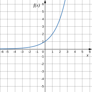 Answer: This function is a combination of three transformations:
1. a vertical reflection:
[latex]f(-x)=2^{-x}[/latex]
2. followed by a reflection in the horizontal axis:
[latex]-f(-x)=-2^{-x}[/latex]
3. followed by the vertical shift up by 1:
[latex]-f(-x)+1=-2^{-x}+1[/latex].
We can sketch a graph by applying these transformations one at a time to the original function:
|
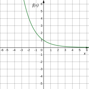 |
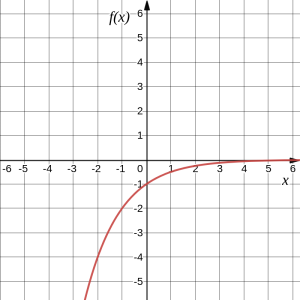 |
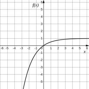 |
| The original graph | Horizontally reflected | Then vertically reflected | Final graph |
Note: As a model for learning, this function would be limited to a domain of [latex]x\geq 0[/latex], with corresponding range [latex][0,1)[/latex].
Vertical stretch/compression
Given a function [latex]f(x)[/latex], if we define a new function [latex]g(x)[/latex] as [latex]g(x)=k\cdot f(x)[/latex], where k is a constant, then [latex]g(x)[/latex] is a vertical stretch or compression of the function [latex]f(x)[/latex].
- If [latex]k \gt 1[/latex], then the graph will be stretched
- If [latex]0\lt k \lt 1[/latex], then the graph will be compressed
- If [latex]k \lt 0[/latex], then there will be combination of a vertical stretch or compression with a vertical reflection
Conversely, if we wish to stretch every point on the graph away from the horizontal axis (or compress it towards the horizontal axis) by a certain factor, effectively we are keeping the horizontal coordinates the same and changing the vertical coordinate by multiplying (or dividing) by the constant factor. Since the horizontal coordinate represents the input of the function and the vertical coordinate represents the output of the function, the input will remain the same while the output value is multiplied (or divided) by the constant.
For example, consider the function
[latex]f(x)=3-\sqrt{2x^2+1}[/latex]
Then stretching this function vertically by, say, a factor of [latex]5[/latex], would result in a new function
[latex]p(x)=5f(x)=5(3-\sqrt{2x^2+1})=15-5\sqrt{2x^2+1}[/latex]
and compressing [latex]f(x)[/latex] vertically by a factor of [latex]5[/latex] would result in yet another function
[latex]q(x)=\frac{1}{5}f(x)=\frac{1}{5}(3-\sqrt{2x^2+1})=\frac{3}{5}-\frac{1}{5}\sqrt{2x^2+1}[/latex]
Example 10
The graph below is a transformation of the function [latex]f(x)=x^3[/latex]. Relate this new function [latex]g(x)[/latex] to [latex]f(x)[/latex], then find a formula for [latex]g(x)[/latex].
![]()
![]() Answer: Recall the graph of [latex]f(x)=x^3[/latex], shown on the right.
Answer: Recall the graph of [latex]f(x)=x^3[/latex], shown on the right.
When trying to determine what transformation(s) took place, it is helpful to look for a point on the graph whose coordinates are relatively easy to determine and whose image is easily located in the graph of the new function.
We first notice that the general shape relative to the origin did not change, i.e, there was no shift horizontally or vertically, nor was there a reflection. However, we notice that the graph of [latex]g[/latex] appears to be vertically "squished" towards the horizontal axis, i.e., vertically compressed.
To determine if that is the case, and by what factor, we pick a point on the graph whose coordinates are relatively easy to determine. In this graph, it appears that [latex]g(2)=2[/latex], yet, at the same input, [latex]f(2)=2^3=8[/latex]. Based on that, it appears that the outputs of [latex]g[/latex] may be [latex]\frac{1}{4}[/latex] of the outputs of the function [latex]f[/latex], since [latex]g(2)=\frac{1}{4}f(x)[/latex]. We can do a test on few more points comparing [latex]g(x)[/latex] to [latex]f(x)[/latex] and this would show that indeed we can fairly safely conclude that [latex]g(x)=\frac{1}{4}f(x).[/latex]
We can write a formula for [latex]g[/latex] by using the definition of the function [latex]f[/latex]: [latex]g(x)=\frac{1}{4}f(x)=\frac{1}{4}x^3.[/latex]
Visual demonstration:
Follow the links below to see the effect of multiplying the value of [latex]f(x)[/latex] by a parameter [latex]k[/latex]. In this demonstration we use the function [latex]f(x)=x^3[/latex] but you can change it to a function of your choice to explore this transformation in different settings.
Horizontal stretch/compression
Given a function [latex]f(x)[/latex], if we define a new function [latex]g(x)[/latex] as [latex]g(x)=f(k\cdot x)[/latex], where k is a constant, then [latex]g(x)[/latex] is a horizontal stretch or compression of the function [latex]f(x)[/latex].
- If [latex]k \gt 1[/latex], then the graph will be compressed
- If [latex]0\lt k \lt 1[/latex], then the graph will be stretched
- If [latex]k \lt 0[/latex], then there will be combination of a vertical stretch or compression with a vertical reflection
Conversely, if we wish to stretch every point on the graph away from the vertical axis (or compress it towards the vertical axis) by a certain factor, effectively we are keeping the horizontal coordinates the same and changing the vertical coordinate using the given factor. The mathematics of this change requires us to apply this factor counter-intuitively (similar to the horizontal transformation: horizontal shift left/right): if we want to stretch the points away from the vertical axis, we have to divide the input variable by the factor, and if we want to compress it towards the vertical axis, we have to multiply the input by the given factor. Since the horizontal coordinate represents the input of the function and the vertical coordinate represents the output of the function, the input will be divided (or multiplied) by the constant while the output value will remain the same.
For example, consider again the function
[latex]f(x)=3-\sqrt{2x^2+1}[/latex]
Then stretching this function horizontally by, say, a factor of [latex]5[/latex], would result in a new function
[latex]r(x)=f\left(\frac{1}{5}x\right)=3-\sqrt{2\left(\frac{1}{5}x\right)^2+1}=3-\sqrt{\frac{2}{25}x^2+1}[/latex]
and compressing [latex]f(x)[/latex] horizontally by a factor of [latex]5[/latex] would result in yet another function
[latex]s(x)=f(5x)=3-\sqrt{2(5x)^2+1}=3-\sqrt{50x^2+1}[/latex]
Combining Transformations
Since transformations are compositions of functions, when combining transformations, it is very important to consider the order of the transformations. For example, vertically shifting by 3 and then vertically stretching by 2 does not create the same graph as vertically stretching by 2 and then vertically shifting by 3. The order follows from analyzing the order of operations.
Combining Vertical Transformations
When combining vertical transformations written in the form [latex]a\cdot f(x)+k[/latex], first vertically stretch by
[latex]a[/latex], then vertically shift by [latex]k[/latex].
As a rule, when translating an algebraic transformation into a graph, follow the order of operations as they are applied on the input value.
Example 11
Describe the transformation from [latex]f(x)=4^x[/latex] to [latex]g(x)=-4^{x-3}-4[/latex].
Answer:
We will start with [latex]f(x)=4^x[/latex] and transform it step by step following the operations applied on the input and output.
| [latex]f(x)=4^x|[/latex] | ||
| [latex]\quad \big\downarrow[/latex] | ||
| [latex]f_1(x)=4^{x-3}=f(x-3)[/latex] | [latex]\longleftarrow[/latex] | shift [latex]f(x)[/latex] to the right by [latex]3[/latex], followed by |
| [latex]\quad \big\downarrow[/latex] | ||
| [latex]f_2(x)=4^{x-3}=-f_1(x)[/latex] | [latex]\longleftarrow[/latex] | reflection of [latex]f_1(x)[/latex] in the horizontal axis, followed by |
| [latex]\quad \big\downarrow[/latex] | ||
| [latex]f_3(x)=-4^{x-3}-4=f_2(x)-4[/latex] | [latex]\longleftarrow[/latex] | shift [latex]f_2(x)[/latex] down by [latex]4[/latex] |
| Therefore, | ||
| [latex]g(x)=-4^{x-3}-4=f_2(x)-4=f_3(x)[/latex] | [latex]\longleftarrow[/latex] | shift [latex]f(x)[/latex] to the right by [latex]3[/latex], then the reflection in the [latex]x[/latex]-axis, and then down by [latex]4[/latex] |
Example 12
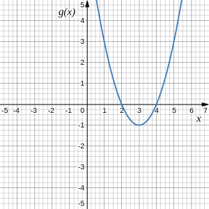
Write an equation for the graph shown as a transformation of the quadratic function [latex]g(x)=x^2[/latex].
![]()
![]() Answer: Since [latex]g(x)[/latex] is the basic quadratic function, first consider what the basic quadratic kit function looks like and how this has changed. Recall the graph of [latex]g(x)=x^2[/latex], plotted on the right.
Answer: Since [latex]g(x)[/latex] is the basic quadratic function, first consider what the basic quadratic kit function looks like and how this has changed. Recall the graph of [latex]g(x)=x^2[/latex], plotted on the right.
Observing the two graphs, we notice several transformations: The basic quadratic function has been flipped over the [latex]x[/latex] axis, and we can see a shift to the right 3 units and a shift up 1 unit. It is not yet clear if some kind of stretch or compression has occurred.
Let's try to plot these transformations one by one:
| [latex]\to[/latex] | [latex]\to[/latex] | [latex]\to[/latex] | [latex]\to[/latex] | |||||
| original | reflection in the [latex]x[/latex]-axis | shift right by 3 | shift up by 1 | vertical stretch by factor of 2 | ||||
| [latex]g(x)=x^2[/latex] | [latex]h(x)[/latex] | [latex]k(x)[/latex] | [latex]l(x)[/latex] | [latex]f(x)[/latex] |
where, starting with [latex]g(x)=x^2[/latex] we have:
- Vertical reflection [latex]\to h(x)=-g(x)=-x^2[/latex]; followed by
- Horizontal shift right by 3 units [latex]\to k(x)=h(x-3)=-(x-3)^2[/latex]; followed by
- Vertical shift up by 1 unit [latex]\to l(x)=k(x)+1=-(x-3)^2+1[/latex]; followed by
- Vertical stretch by factor of 2 [latex]\to f(x)=2l(x)=2(-(x-3)^2+1)[/latex]
Thus the function that produces the given graph is [latex]f(x)=-2(x-3)^2+2.[/latex]
Exercises
Work on the following exercises. Discuss your solutions with your peers and/or course instructor.
IC4NITS Exercises 1.3 - Operations on Functions
