2.2 The Derivative
2.2 The Derivative
In life, whether for work or for pleasure or just plain existence, we are constantly answering one of the three following questions:
- If I (or so-and-so) do this, what will be the outcome?
- If I (or so-and-so) change this from one thing to another thing, how will the outcome change?
- If I (or so-and-so) am changing this in a certain way, what will be the effect on the outcome?
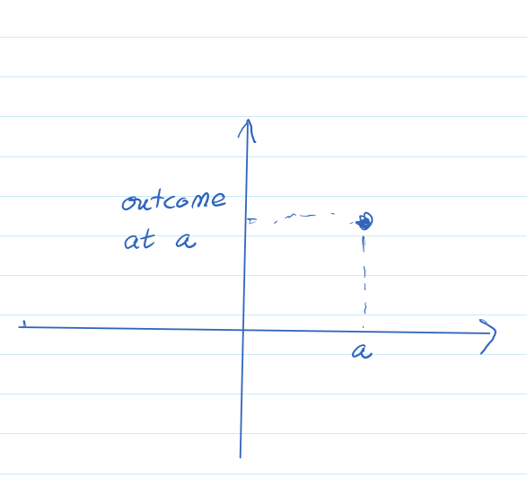
The first question boils down evaluation of some rule we have defined that describes the relationship between the outcome and whatever we are doing. This rule can be a function in the sense we have discussed functions so far, where each input has only one output, or it could be more vague, where there are different possibilities of outcome given a singular input, in which case we tend to associate probabilities of each outcome, the subject of the study of probability and statistics, including expansion of our notion of functions to so-called multivariate functions. In either case, this first questions addresses the question of the value of the outcome at a singular input.
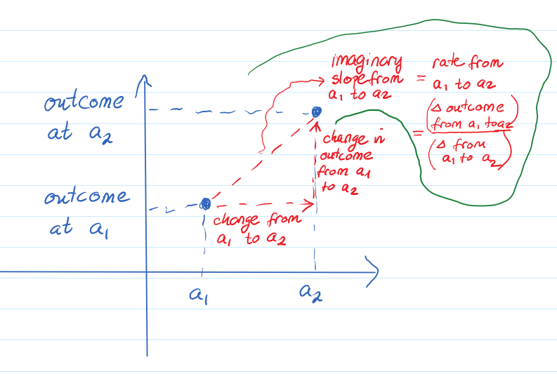
In the second question, "if I (or so-and-so) change this from one thing to another thing, how will the outcome change", we are not looking at a singular point but at two points, evaluating the relationship between the change in the outcome, or the output, in relation to changing the input. This relationship is most often considered in terms of a rate, as in a ratio of the change in the outcome vs. change in the incoming values., i.e., change in output per given change in input, but it is conditional on knowing the start and end point of the change we are looking at. For example, we may want to know the specific amount by which the upload speed increases when the file size increases from one specific value to another specific value and we may want to approximate this change in relation to particular increments of change on this interval, as in, "the upload speed on average increases by ___ per ___ file size".
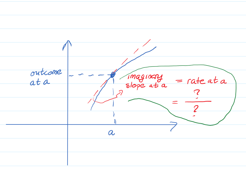
The last question talks about change in the moment, which is a bit weird because how can we consider the question of change if we don't have the start and the end point? This is where the instantaneous rate of change comes in, the bread and butter of calculus, where we are looking at how fast (or slow) the outcome is increasing or decreasing (or not changing at all) if we consider increasing (or decreasing) the incoming values. Note the use of -ing verb endings in this type of change - we use the present participle verb tense because we are talking about something happening in a given moment.
 |
 |
 |
The idea of slope at a point
The slope of a line measures how fast a line rises or falls as we move from left to right along the line. It measures the rate of change of the vertical coordinate (the output) with respect to changes in the horizontal coordinate (the input). If the line represents the distance traveled over time, for example, then its slope represents the velocity. Using the figure below, you can remind yourself of how we calculate slope using two points on the line:
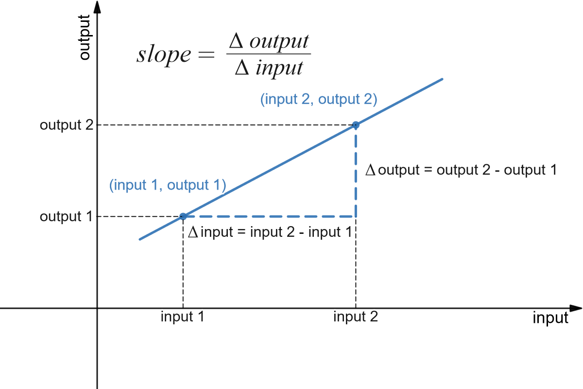 We can also think of slope in contextual, not visual terms. Contextually, the slope represents the rate of change in output in relation to the change in input. The value of slope will tell us whether the line connecting the two points is flat (slope value is zero) or going up (slope value is positive) or going down (slope value is negative). It will also tell us the amount of vertical change over one horizontal unit. To summarize, in the context of rate of change, this value will tell us how, and by how much, the output is changing, on average, with respect to change in one unit of input.
So, when we talk about the slope, we are talking about the slope between two points. Equivalently, when we talk about rate of change, we are talking about two input-output pairs and how the change from one to the other can be described. Therefore, to talk about a slope, we always need two pairs of input-output vales.
However, if you are walking up a hill, or walking down a hill and you stop, you'll still think of being on "a steep slope" or "a gentle slope" even though the hill you are on is not a straight line. Note that when you are thinking about the slope at the point where you are standing, this is not specific to a slope between two specific points on the hill. So where does that sense of slope on a hill come from? It comes from approximating the steepness (and the direction, as in up or down) by your brain picking two imaginary points close to where you are standing and then getting a rough estimate of slope. This concept, of being able to calculate slope at a single point without a reference to some other specific point, is fundamentally behind the concept of "instantaneous rate of change" and that we will discuss throughout this chapter.
Suppose we would like to be able to get that same sort of information about slope (how fast the curve rises or falls, velocity from distance covered over time, etc.) even if the graph is not a straight line. What happens if we try to find the slope of a curve with only one point, as in the figure below?
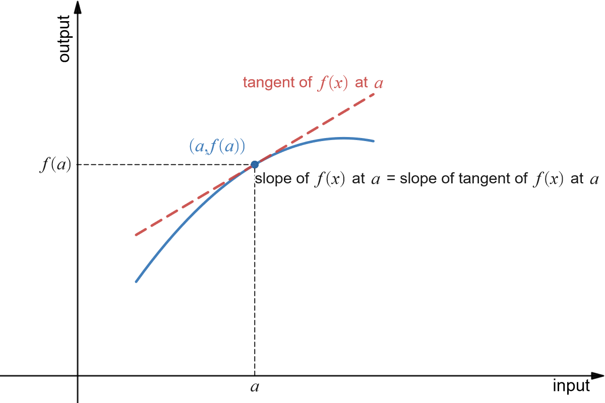 Knowing that we need two points in order to determine the slope of a line, how can we find a slope of a curve at just one point?
The answer, as suggested in the figure, is to find the slope of the tangent line to the curve at that point. Most of us have an intuitive idea of what a tangent line is. Unfortunately, “tangent line” is hard to define precisely and we will use another type of line, the secant line (pronounced as "see-cant") to help us get to the tangent:
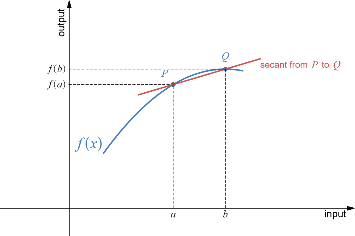
A secant line is a (straight) line between two points on a curve.
We often refer to the secant line simply as the secant.
Here is a visual of a secant line between some two arbitrary points [latex]P[/latex] and [latex]Q[/latex].:Go
 Going back to the idea of the tangent line as the line at a point that imitates the slope of the curve at that point, we will now use secants to build such a line.
Let's try to build the tangent line at point [latex]P[/latex] in the image above. Consider a series of secants going through [latex]P[/latex] and points close to [latex]P[/latex]. As you may be able to see in the image below, the closer the point [latex]Q[/latex] is to the point [latex]P[/latex] (numbered [latex]Q_1[, Q_2, \ldots[/latex]), the closer the secant slope gets to the tangent slope. This idea will be key to finding the tangent slope, but first we need to more carefully define the idea of "getting closer to.
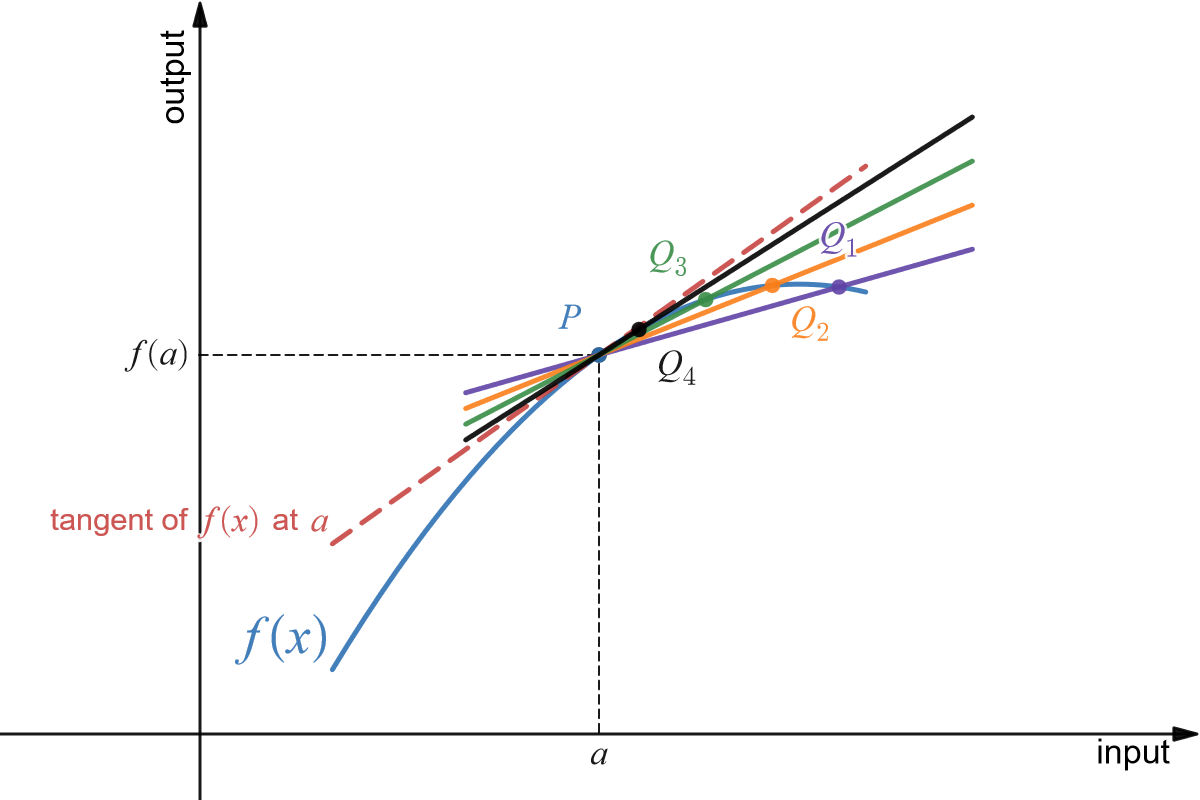
For a dynamic visual, explore this interactive demo: tangent as a limit of secants
Definition of the Derivative
When working with linear functions, we could find the slope of a line to determine the rate at which the function is changing. For an arbitrary function, we can determine the average rate of change of the function. This is the slope of the secant line through those two points on the graph.
Average Rate of Change
= the slope of the secant line through the two points [latex]\left(a, f(a)\right)[/latex] and [latex]\left(b, f(b)\right)[/latex]
Example 1
Suppose the total cost of producing [latex]x[/latex] items is given by [latex]C(x) = 200+30x-0.1x^2[/latex]. Determine the average rate of change of cost when increasing production from 25 units to 100 units.
Answer: average rate of change in cost from 25 to 100 units?
[latex]\begin{align*} \text{average rate of change in cost from 25 to 100 units}&=\dfrac{\overset{?}{C(100)}-\overset{?}{C(25)}}{100-25}\\\\ &=\dfrac{(200+30(100)-0.1(100)^2)-(200+30(25)-0.1(25)^2)}{100-25}\\\\&=$17.50\text{ per unit}\end{align*}[/latex]
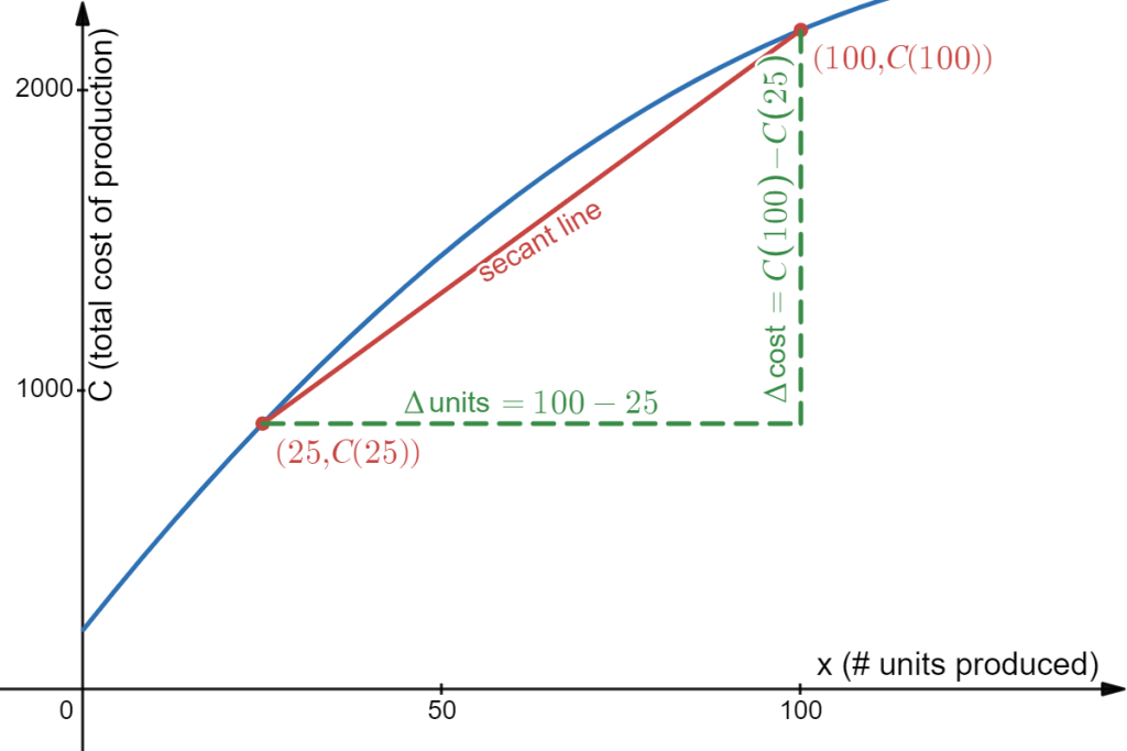
The average rate of change is the slope of the secant line between (25, 887.50) and (100, 2200). Since its value is the positive 17.50, this tells us that, on average, the cost increases by $17.50 for each unit produced.
Visually we can represent this situation by:
Thinking about the last example, suppose instead we asked the question "How fast are costs increasing when production is 25 units?" Notice this is a different kind of question. The question in the example asked for the rate of change over an interval, as production increased from one value to another. The new question is again asking for a rate of change, but an instantaneous rate of change, at a particular moment.
We don’t yet have a way to calculate the rate of change except over an interval. In the next example we will explore a couple ways to estimate the instantaneous rate of change.
Example 2
Suppose the total cost of producing [latex]x[/latex] items is given by [latex]C(x) = 200+30x-0.1x^2[/latex]. Estimate the instantaneous rate of change at the production level of 25 items.
Answer:
We can see in the previous graph that the secant slope on the interval [latex]25\le x \le 100[/latex] is not a particularly good estimate of the instantaneous rate of change since the cost function seems steeper at [latex]x = 25[/latex] than the secant line. We could improve the estimate by choosing a smaller interval, taking another production level that is closer to the production level of 25 items.
Approach 1: Using smaller intervals
Using the interval [latex]25\le x \le 30[/latex], the average rate of change would be:
[latex]\frac{C(30) - C(25)}{30 - 25} = \frac{(200+30(30)-0.1(30)^2)-(200+30(25)-0.1(25)^2-}{30-25} = $24.50 \text{ per unit}[/latex]
Using an interval on the other side, [latex]20\le x \le 25[/latex], the average rate of change would be:
[latex]\frac{C(25) - C(20)}{25 - 20} = \frac{(200+30(25)-0.1(25)^2)-(200+30(20)-0.1(20)^2}{25-20} = $25.50 \text{ per unit}[/latex]
Visually, we can see both these secant lines seem to approximate the function pretty well.
We would expect the instantaneous rate of change to be somewhere between these two values. Averaging them, we get an estimate of $25 per unit for the instantaneous rate of change.
Approach 2: Estimating from the graph.
This approach is more commonly used when we only have the graph of a function, and don’t have a formula to evaluate, but we will illustrate it here using the same function.
The instantaneous rate of change at a point is the slope of the tangent line at that point, which is the line that passes through the point and has the same rate of change (slope) as the function does at the point. Given a graph, we can sketch in a tangent line by holding a ruler up to the graph, and drawing in a line that touches the graph when [latex]x = 25[/latex] and approximately has the same slope.
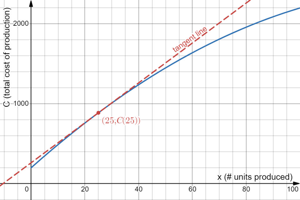
To estimate the instantaneous rate of change, we can now calculate the slope of this drawn-in line. Looking at the graph, the tangent line appears to pass approximately through (30, 1000) and (70, 2000) which would give a slope of [latex]\frac{2000-1000}{70-30}=\frac{1000}{40}=25[/latex] dollars per unit.
Note that neither of the approaches gives us the exact rate of change at [latex]x=25[/latex]. For that, we need the notion of the derivative and tools to calculate it, when possible.
Video Demonstration
Instantaneous rate of change and tangent lines
© 2014 Eric Bancroft
In the previous examples, we noticed that as the interval got smaller and smaller, the secant line got closer to the tangent line and its slope got closer to the slope of the tangent line. That’s good news – we know how to find the slope of a secant line.
Let's explore further this idea of finding the tangent slope based on the secant slope.
Example 3
Find the slope of the line [latex]L[/latex] in the graph below which is tangent to [latex]f(x) = x^2[/latex] at the point (2,4).
Answer:
We could estimate the slope of [latex]L[/latex] from the graph, but we won't. Instead, we will use the idea that secant lines over tiny intervals approximate the tangent line.
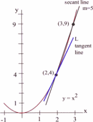
We can see that the line through (2,4) and (3,9) on the graph of [latex]f[/latex] is an approximation of the slope of the tangent line, and we can calculate that slope exactly: [latex]m = \frac{\Delta y}{\Delta x} = \frac{9-4}{3-2} = 5[/latex]. But [latex]m = 5[/latex] is only an estimate of the slope of the tangent line and not a very good estimate. It's too big. We can get a better estimate by picking a second point on the graph of [latex]f[/latex] which is closer to (2,4) – the point (2,4) is fixed and it must be one of the points we use.
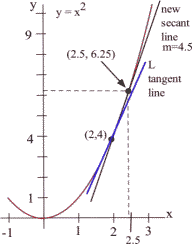
From the second figure, we can see that the slope of the line through the points (2,4) and (2.5,6.25) is a better approximation of the slope of the tangent line at (2,4):
[latex]m = \frac{\Delta y}{\Delta x} = \frac{6.25 - 4}{2.5 - 2} = \frac{2.25}{0.5} = 4.5[/latex]
This is a better estimate, but still an approximation. We can continue picking points closer and closer to (2,4) on the graph of [latex]f[/latex], and then calculating the slopes of the lines through each of these points and the point (2,4):
Points to the left of (2,4)
| [latex]x[/latex] | [latex]y=x^2[/latex] | Slope of line through [latex](x,y)[/latex] and [latex](2,4)[/latex] |
| 1.5 | 2.25 | 3.5 |
| 1.9 | 3.61 | 3.9 |
| 1.99 | 3.9601 | 3.99 |
Points to the right of (2,4)
| [latex]x[/latex] | [latex]y=x^2[/latex] | Slope of line through [latex](x,y)[/latex] and [latex](2,4)[/latex] |
| 3 | 9 | 5 |
| 2.5 | 6.25 | 4.5 |
| 2.01 | 4.0401 | 4.01 |
The only thing special about the x–values we picked is that they are numbers which are close, and very close, to [latex]x = 2[/latex]. Someone else might have picked other nearby values for [latex]x[/latex]. As the points we pick get closer and closer to the point [latex](2,4)[/latex] on the graph of [latex]y = x^2[/latex], the slopes of the lines through the points and [latex](2,4)[/latex] are better approximations of the slope of the tangent line, and these slopes are getting closer and closer to [latex]4[/latex].
We can bypass much of the calculating by not picking the points one at a time: let's look at a general point near [latex](2,4)[/latex]. Define [latex]x = 2 + h[/latex] so [latex]h[/latex] is the increment from [latex]2[/latex] to [latex]x[/latex]. If [latex]h[/latex] is small, then [latex]x = 2 + h[/latex] is close to [latex]2[/latex] and the point [latex](2+h, f(2+h) ) = \left(2+h, (2+h)^2\right)[/latex] is close to [latex](2,4)[/latex].
The slope [latex]m[/latex] of the line through the points [latex](2,4)[/latex] and [latex]\left(2+h, (2+h)^2\right)[/latex] is a good approximation of the slope of the tangent line at the point (2,4):
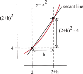
[latex]m=\dfrac{(2+h)^2-4}{(2+h)-2}=\dfrac{\left(4+4h+h^2\right)-4}{h}=\dfrac{4h+h^2}{h}=\dfrac{h(4+h)}{h}=4+h[/latex]
The value [latex]m = 4 + h[/latex] is the slope of the secant line through the two points [latex](2,4)[/latex] and [latex]\left( 2+h, (2+h)^2 \right)[/latex]. As [latex]h[/latex] gets smaller and smaller, this slope approaches the slope of the tangent line to the graph of [latex]f[/latex] at [latex](2,4)[/latex].
More formally, we could write:
[latex]\text{Slope of the tangent line} = \dfrac{\Delta y}{\Delta x} = \lim\limits_{h\to 0} (4+h).[/latex]
We can easily evaluate this limit using direct substitution, finding that as the interval [latex]h[/latex] shrinks towards [latex]0[/latex], the secant slope approaches the tangent slope, [latex]4[/latex].
Finding tangent slopes and finding the instantaneous rate of change are the same problem. In each problem we wanted to know how rapidly something was changing at an instant in time , and the answer turned out to be finding the slope of a tangent line, which we approximated with the slope of a secant line. This idea is the key to defining the slope of a curve.
Video Demonstration
Example: finding the equation of tangent line
© 2014 Eric Bancroft
The Derivative
Meaning of the derivative
We can view the derivative in different ways. Here are a three of them:
- The derivative of a function [latex]f[/latex] at a point [latex](a, f(a))[/latex] is the instantaneous rate of change in [latex]f(x)[/latex] at [latex]a[/latex].
- The derivative of [latex]f[/latex] at [latex]a[/latex] is the slope of the tangent line to the graph of [latex]f[/latex] at the point [latex](a, f(a))[/latex].
- The derivative of [latex]f[/latex] at [latex]a[/latex] is the slope of the curve [latex]f(x)[/latex] at the point [latex](a, f(a))[/latex].
A function [latex]f[/latex] is said to be differentiable at [latex]a[/latex] if its derivative exists at [latex](a, f(a))[/latex].
Notation for the Derivative
The derivative of [latex]y=f(x)[/latex] can symbolically be written in different ways, all meaning the same thing but providing different levels of detail:
- [latex]f'(x)[/latex] (read aloud as "[latex]f[/latex] prime of [latex]a[/latex]")
- [latex]y'[/latex] (read aloud as "why prime")
- [latex]\frac{dy}{dx}[/latex] (read aloud as "dee why dee ex"), or [latex]\frac{df}{dx}.[/latex]
The notation that resembles a fraction is called Leibniz notation. It displays not only the name of the function ([latex]f[/latex] or [latex]y[/latex]), but also the name of the variable (in this case, [latex]x[/latex]). It looks like a fraction because the derivative is a slope however it is not a fraction.
Formal Algebraic Definition
[latex]f'(x)=\lim\limits_{h\to 0} \dfrac{f(x+h)-f(x)}{h}[/latex]
Practical Definition
The derivative can be approximated by looking at an average rate of change, or the slope of a secant line, over a very tiny interval. The tinier the interval, the closer this is to the true instantaneous rate of change, slope of the tangent line, or slope of the curve.
When determining the value (or the function) of the derivative, we use the following expressions to describe that task:
- Find the derivative of a function
- Take the derivative of a function
- Differentiate a function
We use an adaptation of the [latex]\frac{df}{dx}[/latex] notation to mean "find the derivative of [latex]f(x)[/latex]":
[latex]\dfrac{d}{dx}\left(f(x))\right]=\frac{df}{dx}[/latex]
In the next section we will learn methods for computing exact values of derivatives from formulas rather than calculating the derivative as a limit. If the function is given to you as a table or graph, you will still need to approximate this way.
This is the foundation for the rest of this chapter. It’s remarkable that such a simple idea (the slope of a tangent line) and such a simple definition (for the derivative [latex]f'(x)[/latex]) will lead to so many important ideas and applications.
Example 4
Find the slope of the tangent line to [latex]f(x)=\frac{1}{x}[/latex] at [latex]x = 3[/latex].
Answer:
The slope of the tangent line is the value of the derivative [latex]f'(3)[/latex]. [latex]f(3)=\frac{1}{3}[/latex] and [latex]f(3+h)=\frac{1}{3+h}[/latex], so, using the formal limit definition of the derivative, [latex]f'(3)=\lim\limits_{h\to 0}\frac{f(3+h)-f(3)}{h}=\lim\limits_{h\to 0}\frac{\frac{1}{3+h}-\frac{1}{3}}{h}.[/latex]
We can simplify by giving the fractions a common denominator:
[latex]\begin{align*} \lim\limits_{h\to 0}\frac{\frac{1}{3+h}-\frac{1}{3}}{h} & = \lim\limits_{h\to 0}\frac{\frac{1}{3+h}\cdot\frac{3}{3}-\frac{1}{3}\cdot\frac{3+h}{3+h}}{h} \\ & = \lim\limits_{h\to 0}\frac{\frac{3}{9+3h}-\frac{3+h}{9+3h}}{h} \\ & = \lim\limits_{h\to 0}\frac{\frac{3-(3+h)}{9+3h}}{h} \\ & = \lim\limits_{h\to 0}\frac{\frac{3-3-h}{9+3h}}{h} \\ & = \lim\limits_{h\to 0}\frac{\frac{-h}{9+3h}}{h} \\ & = \lim\limits_{h\to 0}\frac{-h}{9+3h}\cdot\frac{1}{h} \\ & = \lim\limits_{h\to 0}\frac{-1}{9+3h} \\ \end{align*}[/latex] and the evaluate using direct substitution: [latex]\lim\limits_{h\to 0}\frac{-1}{9+3h}=\frac{-1}{9+3(0)}=-\frac{1}{9}.[/latex]
Thus, the slope of the tangent line to [latex]f(x)=\frac{1}{x}[/latex] at [latex]x = 3[/latex] is [latex]-\frac{1}{9}[/latex].
The Derivative as a Function
We now know how to find (or at least approximate) the derivative of a function for any [latex]x[/latex]-value; this means we can think of the derivative as a function, too. The inputs are the same [latex]x[/latex]’s; the output is the value of the derivative at that [latex]x[/latex] value.
Example 5
Below is the graph of a function [latex]y=f(x)[/latex]. We can use the information in the graph to fill in a table showing values of [latex]f'(x):[/latex]
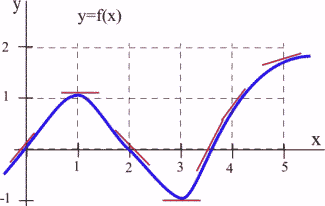
Answer:
At various values of [latex]x[/latex], draw your best guess at the tangent line and measure its slope. You might have to extend your lines so you can read some points. In general, your estimate of the slope will be better if you choose points that are easy to read and far away from each other. Here are estimates for a few values of [latex]x[/latex] (parts of the tangent lines used are shown above in the graph):
| [latex]x[/latex] | [latex]y=f(x)[/latex] | [latex]f'(x)=[/latex] the estimated slope of the tangent line to the curve at the point [latex](x,y)[/latex]. |
| 0 | 0 | 1 |
| 1 | 1 | 0 |
| 2 | 0 | -1 |
| 3 | -1 | 0 |
| 3.5 | 0 | 2 |
We can estimate the values of [latex]f'(x)[/latex] at some non-integer values of [latex]x[/latex], too: [latex]f'(0.5) \approx 0.5[/latex] and [latex]f'(1.3) \approx -0.3[/latex].
We can even think about entire intervals. For example, if [latex]0 \lt x \lt 1[/latex], then [latex]f(x)[/latex] is increasing, all the slopes are positive, and so [latex]f'(x)[/latex] is positive.
The values of [latex]f'(x)[/latex] definitely depend on the values of [latex]x[/latex], and [latex]f'(x)[/latex] is a function of [latex]x[/latex]. We can use the results in the table to help sketch the graph of [latex]f'(x)[/latex].
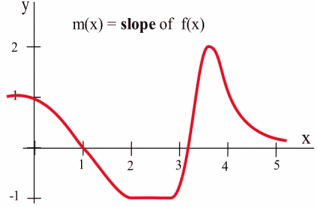
To get a better feel for this, explore the interactive demo below. Drag the point slider to change the point a and notice how the slope of the tangent line corresponds to the value of the derivative [latex]f'(x)[/latex].
Example 6
Shown is the graph of the height [latex]h(t)[/latex] of a rocket at time [latex]t[/latex].
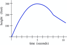
Answer:
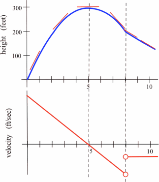
Sketch the graph of the velocity of the rocket at time [latex]t[/latex]. (Velocity is the derivative of the height function, so it is the slope of the tangent to the graph of position or height.)
We can estimate the slope of the function at several points. The lower graph below shows the velocity of the rocket. This is [latex]v(t) = h'(t)[/latex].
In some applications, we need to know where the graph of a function f(x) has horizontal tangent lines (slopes = 0).
Example 9
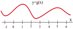
Below is the graph of [latex]y = g(x)[/latex]. At what values of [latex]x[/latex] does the graph of [latex]g(x)[/latex] have horizontal tangent lines?
Answer:
The tangent lines to the graph of [latex]g(x)[/latex] are horizontal (slope = 0) when [latex]x\approx -1, 1, 2.5, \text{ and } 5[/latex].
We can also find derivative functions algebraically using limits.
Example 10
Find [latex]\frac{d}{dx}\left( 2x^2-4x-1 \right)[/latex].
Answer:
Setting up the derivative using a limit, [latex]f'(x)=\lim\limits_{h\to 0}\frac{f(x+h)-f(x)}{h}.[/latex]
We will start by simplifying [latex]f(x+h)[/latex] by expanding:
[latex]\begin{align*} f(x+h) & = 2(x+h)^2-4(x+h)-1 \\ & = 2(x^2+2xh+h^2)-4(x+h)-1 \\ & = 2x^2+4xh+2h^2-4x-4h-1 \end{align*}[/latex]
Now finding the limit:
[latex]\begin{align*} f'(x) & = \lim\limits_{h\to 0}\frac{f(x+h)-f(x)}{h} \\ & = \lim\limits_{h\to 0} \frac{(2x^2+4xh+2h^2-4x-4h-1)-(2x^2-4x-1)}{h} \\ & = \lim\limits_{h\to 0} \frac{2x^2+4xh+2h^2-4x-4h-1-2x^2+4x+1}{h} \qquad \text{(Substitute in the formulas.)} \\ & = \lim\limits_{h\to 0} \frac{4xh+2h^2-4h}{h} \qquad \text{(Now simplify.)}\\ & = \lim\limits_{h\to 0} \frac{h(4x+2h-4)}{h} \qquad \text{(Factor out the }h\text{, then cancel.)} \\ & = \lim\limits_{h\to 0} (4x+2h-4) \end{align*}[/latex]
We can find the limit of this expression by direct substitution:
[latex]f'(x)=\lim\limits_{h\to 0} (4x+2h-4)=4x-4[/latex]
Note that the derivative depends on [latex]x[/latex], and that this formula will tell us the slope of the tangent line to [latex]f[/latex] at any value [latex]x[/latex]. For example, if we wanted to know the tangent slope of [latex]f[/latex] at [latex]x = 3[/latex], we would simply evaluate: [latex]f'(3)=4(3)-4=8[/latex].
A formula for the derivative function is very powerful, but as you can see, calculating the derivative using the limit definition is very time consuming. In the next section, we will identify some patterns that will allow us to start building a set of rules for finding derivatives without needing the limit definition.
Interpreting the Derivative
So far we have emphasized the derivative as the slope of the line tangent to a graph. That interpretation is very visual and useful when examining the graph of a function, and we will continue to use it. Derivatives, however, are used in a wide variety of fields and applications, and some of these fields use other interpretations. The following are a few interpretations of the derivative that are commonly used.
General
Rate of Change: [latex]f '(x)[/latex] is the rate of change of the function at [latex]x[/latex]. If the units for [latex]x[/latex] are years and the units for [latex]f(x)[/latex] are people, then the units for [latex]\frac{df}{dx}[/latex] are [latex]\frac{\text{people}}{\text{year}}[/latex], a rate of change in population.
Graphical
Slope: [latex]f '(x)[/latex] is the slope of the line tangent to the graph of [latex]f[/latex] at the point [latex]( x, f(x) )[/latex] .
Physical
Velocity: If [latex]f(x)[/latex] is the position of an object at time [latex]x[/latex], then [latex]f '(x)[/latex] is the velocity of the object at time [latex]x[/latex] because velocity measures the change in distance over time at a particular moment. If the units for [latex]x[/latex] are hours and [latex]f(x)[/latex] is distance measured in kilometers, then the units for [latex]f '(x) = \frac{df}{dx}[/latex] are kilometer/hour, or km/h. Note that velocity is different from speed. Speed only gives information on how fast, whereas velocity also gives information about the direction. For example, if the velocity is a negative number, then that means that the change in position is negative, i.e., the object is going backwards.
Acceleration: If [latex]f(x)[/latex] is the velocity of an object at time [latex]x[/latex], then [latex]f '(x)[/latex] is the acceleration of the object at time [latex]x[/latex]. If the units are for [latex]x[/latex] are hours and [latex]f(x)[/latex] has the units kilometer/hour, then the units for the acceleration [latex]f '(x) = \frac{df}{dx}[/latex] are (kilometer/hour)/hour, i.e., kilometer/hour2, or kilometers per hour per hour.
One of the strengths of calculus is that it provides a unity and economy of ideas among diverse applications. The vocabulary and problems may be different, but the ideas and even the notations of calculus are still useful. We will see this in more contextual situations in the units ahead.
Concept Check
Test your understanding: Meaning of Derivatives
Section Exercises
Work on the following exercises. Discuss your solutions with your peers and/or course instructor.
IC4NITS Exercises 2.2 - Derivatives
