2.7: Maxima and Minima
2.7: Maxima and Minima
In this section and the sections that follow, we will discuss a series of calculus tools that will allow us to analyze the behaviour of a function and represent it visually through its graph. These tools will also allow us to tackle optimization problems by modeling them using a function and determining when the function reaches the optimal value, be it the highest or the lowest.
Sign charts
We start by reminding ourselves of the Intermediate Value Theorem:
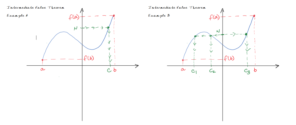
Intermediate Value Theorem
Suppose that [latex]f[/latex] is a continuous function on the closed interval [latex][a, b][/latex] and let [latex]N[/latex] be any number between [latex]f(a)[/latex] and [latex]f(b)[/latex], where [latex]f(a)\neq f(b)[/latex]. Then there exists a number [latex]c\in(a,b)[/latex] such that [latex]f(c)=N[/latex].
Proof: Too difficult for this course.
This theorem becomes quite useful in situations where we are looking for zeros of a function but we cannot determine them using the usual tools such as factoring.
Visually this theorem may seem obvious, as in the two examples above. However, mathematically it is far from obvious and requires a rigorous proof that relies on specific, generally-accepted properties of real numbers such as the completeness axiom. We don't show a proof here but you can review proofs provided in more advanced calculus textbooks or, for example, on Wikipedia, one of which takes the approach of reducing the statement to the following special case:
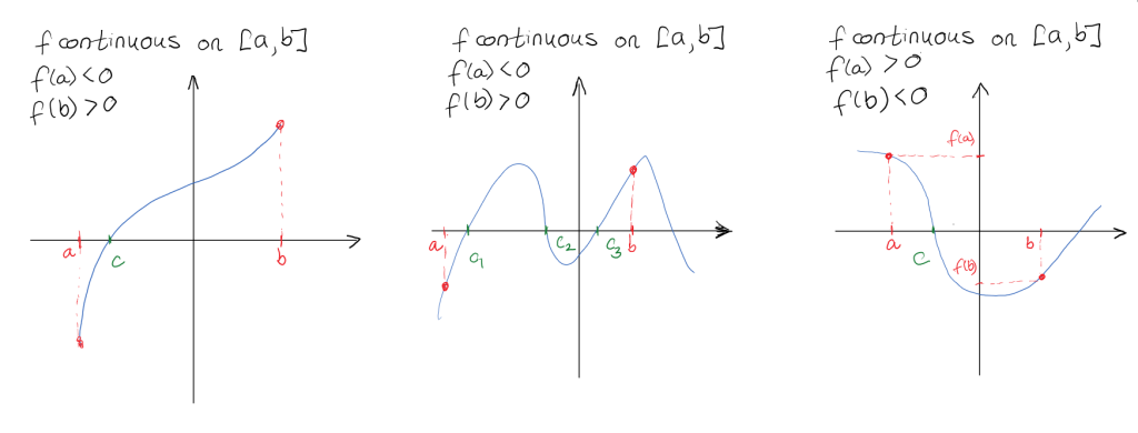
Special case of the Intermediate Value Theorem (Bolzano's Theorem):
If [latex]f[/latex] is continuous on some closed interval [latex][a, b][/latex] and [latex]f(a)<0[/latex] while [latex]f(b)>0[/latex] (or vice versa), then [latex]f[/latex] has a horizontal intercept, i.e., there is a value [latex]c[/latex] for which [latex]f(c)=0[/latex].
For example, we can use Intermediate Value Theorem to demonstrate that
[latex]f(x)=4x^3-6x^2+3x-2[/latex]
has a zero (a horizontal intercept) somewhere on the interval [latex](1, 2)[/latex].
This is true because [latex]f(x)[/latex] is a polynomial, and so it is a continuous function on the interval [latex][1, 2][/latex]. Since [latex]f(1)=-1\lt 0[/latex] and [latex]f(2)=12\gt 0[/latex], by the Intermediate Value Theorem there is a value [latex]c\in(1,2)[/latex] such that [latex]f(c)=0[/latex].
Note that we don't know what that value is; we only know that it exists. If factoring fails us, we could potentially use Newton's Method of Approximation, which uses derivatives to get a close approximation, a method we will discuss later in the course.
In other words, we can use the Intermediate Value Theorem to demonstrate that a function has a zero, but we cannot use it to determine the values of its zeros, if they exists.
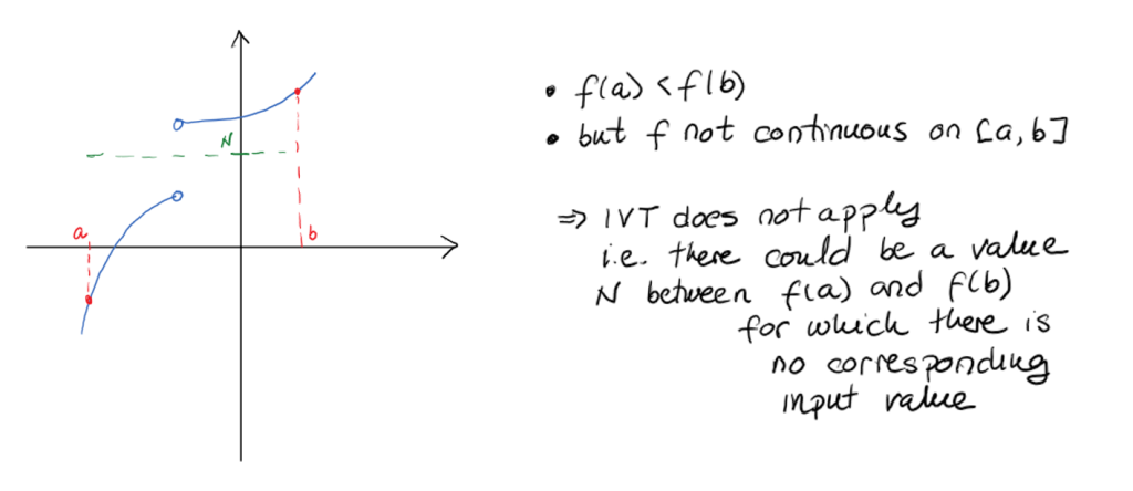
Note that there are three conditions involved in the Intermediate Value Theorem: continuity, on a closed interval, and with different values of the function on the boundaries of the interval. The closed interval condition is necessary if we're to be able to compare the values of the function at the end of the interval. The different values on the interval boundary are necessary if we are to be able to pick an arbitrary number between two values of the function. In addition, the condition of continuity is necessary because otherwise the theorem statement may not be true, as in the visual example below:
For us, one of the most important implications of the Intermediate Value Theorem is the following assertion:
Corollary to Bolzano's Theorem:
If [latex]f[/latex] is a continuous function on on an open interval [latex](a,b)[/latex] where [latex]f(x)\neq 0[/latex] for all [latex]x\in (a,b)[/latex], then [latex]f(x)[/latex]is either always positive on [latex](a,b)[/latex] or always negative on [latex](a,b)[/latex].
Proof: We will demonstrate the truth of this statement using the proof by contradiction method.
Let [latex]f[/latex] be a continuous function on an open interval [latex](a,b)[/latex] where [latex]f(x)\neq 0[/latex] for all [latex]x\in (a,b)[/latex]. Suppose that [latex]f[/latex] is not strictly positive or strictly negative on the open interval [latex](a,b)[/latex]. Then there exist [latex]c[/latex] and [latex]d[/latex] in [latex](a,b)[/latex] such that [latex]f(c)<0[/latex] and [latex]f(d)>0[/latex] or [latex]f(c)>0[/latex] and [latex]f(d)<0[/latex]. Since [latex]f[/latex] is continuous on [latex][a,b][/latex], it is also continuous on the subinterval [latex][c,d][/latex] and so, by Bolzano's theorem, there exists [latex]x\in(c,d)[/latex] such that [latex]f(x)=0[/latex]. This contradicts the assumption that [latex]f(x)\neq 0[/latex] for all [latex]x\in (a,b)[/latex] and so the assertion of a possibility that [latex]f[/latex] is not strictly positive or strictly negative on the open interval [latex](a,b)[/latex] is false. Therefore, [latex]f[/latex] is either strictly positive or strictly negative on the open interval [latex](a,b)[/latex].
[latex]\blacksquare[/latex]
As a point of information, a corollary is a proposition that follows from one that has already been proved. A theorem is a statement that has been or can be proved, where the proof is a logical argument that is presented through a chain of reasoning using already accepted truths.
Here is a very important example of the application of this corollary:
Example 1
Consider the function
[latex]f(x)=\frac{x(x-2)}{x-4}[/latex]
Determine the intervals on which the function has positive values and the intervals on which the function has negative values.
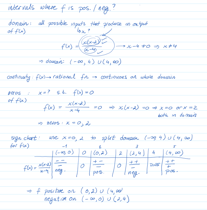
Answer: Intervals where [latex]f(x)[/latex] is positive? Intervals where [latex]f(x)[/latex] is negative?
For a function to have any kind of value, positive or negative, the function has to be defined for the given input. Therefore, we first have to determine the domain of the function, i.e., all possible input values that produce an output, i.e., all values of [latex]x[/latex] such that [latex]f(x)[/latex] can be calculated.
Looking at the definition of this function, we can see that [latex]f(x)[/latex] is calculated first through calculating the numerator which involves subtraction [latex](x-2)[/latex] (which causes no problems), then multiplication [latex]x(x-2)[/latex] (which also causes no problems), then calculating the denominator which involves subtraction ([latex]x-4[/latex]) (again no problems), and then finally division of the numerator by the denominator, which causes a problem only if the denominator is equal to zero. This gives rise to the following condition on [latex]x[/latex]:
[latex]x-4\neq 0\Rightarrow x\neq 4[/latex]
Since this was the only condition on [latex]x[/latex] in obtaining a value for [latex]f(x)[/latex],
domain: [latex](-\infty,4)\cup(4,\infty)[/latex]
To determine the intervals where the function is strictly positive or strictly negative, we look for the values in the domain where the function is zero, then use the zeros to subdivide the domain into sub-intervals on which the function is not zero, so that we can use the corollary to Bolzano's Theorem which tells us that on each of those subintervals, the function is either strictly positive or the function is strictly negative.
First note that [latex]f[/latex] is a rational function, which means that it is continuous on its domain. Therefore the corollary will apply to all subintervals within the domain.
To determine the zeros of [latex]f[/latex] we have to find the values of [latex]x[/latex] in the domain such that [latex]f(x)=0[/latex]. Since [latex]f(x)[/latex] is a quotient, the result will be zero only if the numerator is zero. In other words:
[latex]x(x-2)=0\Leftrightarrow x=0 \text{ or }x-2=0\Leftrightarrow x=0,\ 2[/latex]
Since both [latex]x=0[/latex] and [latex]x=2[/latex] are in the domain of [latex]f[/latex], they are the zeros of [latex]f[/latex]. (Note the significance of the article "the" in "the zeros". It implies these are zeros of [latex]f[/latex] and they are the only zeros of [latex]f[/latex].)
We now partition the domain into sub-intervals using the zeros and determine for each sub-interval whether the function is positive or negative by choosing any value within that sub-interval and evaluating the function at that value. One of the easiest ways of doing this is by creating a so-called sign chart for [latex]f[/latex] and using the factored form of the function (written as a series of multiplications and divisions) to determine the sign (positive or negative) of the function on each of the sub-intervals:
| test value | [latex]-1[/latex] | [latex]1[/latex] | [latex]3[/latex] | [latex]5[/latex] | |||
| [latex]x[/latex] | [latex](-\infty,0)[/latex] | [latex]0[/latex] | [latex](0,2)[/latex] | [latex]2[/latex] | [latex](2,4)[/latex] | [latex]4[/latex] | [latex](4,\infty)[/latex] |
| [latex]f(x)=\dfrac{x(x-2)}{x-4}[/latex] | [latex]\dfrac{--}{-}[/latex] negative |
[latex]0[/latex] | [latex]\dfrac{+-}{-}[/latex] positive |
[latex]0[/latex] | [latex]\dfrac{++}{-}[/latex] negative |
DNE | [latex]\dfrac{++}{+}[/latex] positive |
Therefore, [latex]f[/latex] is positive on [latex](0,2)\cup(4,\infty)[/latex] and negative on [latex](-\infty,0)\cup(2,4)[/latex].
You can visually verify this by plotting the graph of [latex]f[/latex] using a graphing calculator: link to graph. Note that, visually, if the function is positive on an interval, then the graph is above the horizontal axis, and if the function is negative on an interval, the graph is below the horizontal axis.
Here is the same example but solved in hand-written form:
Example 1 (handwritten solution)
Consider the function
[latex]f(x)=\frac{x(x-2)}{x-4}[/latex]
Determine the intervals on which the function has positive values and the intervals on which the function has negative values.
Answer:
It turns out that sign charts will play a large role in our study of the behaviour of a function. Not only will we be interested in the intervals where the function is positive and where it is negative, we will also be interested in determining when its derivative is positive and when it is negative. This is because, as we have learned, knowing that the derivative is positive tells us that the original function is increasing, and the derivative being negative tells us that the function is decreasing, which in turn will tell us when we are at highest points and when we are at lowest points. We will go even further, by creating the sign charts for the second derivative of the function, which will then tell us whether the original function is growing or decaying at an increasing or decreasing rate, i.e., it will allow us to determine the concavity of the function.
Before we get there, however, let's define what we mean by highest and lowest points.
Maximum and minimum values of a function
We define two types of extrema, i.e. values that describe highest and lowest values of a function: absolute and local:
Definition: Let [latex]c[/latex] be a number in the domain [latex]D[/latex] of a function [latex]f[/latex]. Then [latex]f(c)[/latex] is the
- absolute maximum value of [latex]f[/latex] on [latex]D[/latex] if [latex]f(c)≥f(x)[/latex] for all [latex]x\in D[/latex]
- absolute minimum value of [latex]f[/latex] on [latex]D[/latex] if [latex]f(c)≤f(x)[/latex] for all [latex]x\in D[/latex]
- local maximum value of [latex]f[/latex] on [latex]D[/latex] if [latex]f(c)≥f(x)[/latex] when [latex]x[/latex] is near [latex]c[/latex]
- local minimum value of [latex]f[/latex] on [latex]D[/latex] if [latex]f(c)≤f(x)[/latex] when [latex]x[/latex] is near [latex]c[/latex]
These values are also called the extreme values of [latex]f[/latex].
The language minefield: There are two plural forms for a maximum and a minimum. They are maxima or maximums and minima or minimums, respectively. The terms maxima and minima are used mostly in technical communication while the terms maximums and minimums are used in colloquial conversations. Additionally, the absolute extrema (maxima or minima) are also sometimes referred to as global extrema.
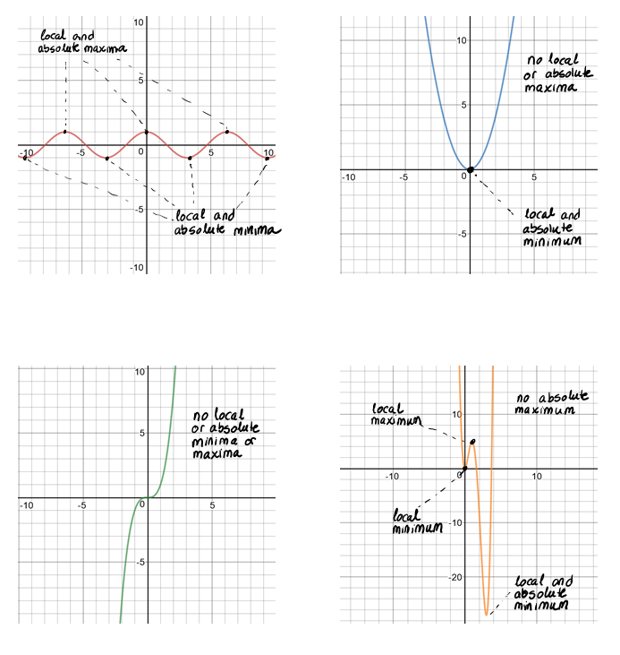
Note that a function can have one or many local and absolute maxima and minima or can have none. Here are some examples:
When investigating the extrema of a function, two questions need to be answered:
- Are there any extrema?
- Where are the extrema?
To answer the first question, that of existence, we often use the Extreme Value Theorem:
Extreme Value Theorem
If [latex]f(x)[/latex] is continuous on a closed interval [latex][a, b][/latex], then [latex]f[/latex] attains an absolute maximum value [latex]f(c)[/latex] and an absolute minimum value [latex]f(d)[/latex] at some numbers [latex]c[/latex] and [latex]d[/latex] in the interval [latex][a, b].[/latex]
Proof: Too difficult for this course.
Important note: this theorem tells us that the absolute maximum and minimum exists on a closed interval of a continuous function. In other words, if we know we are dealing with a function that is continuous on some closed interval, then we know that, on this interval, the function will have an absolute maximum and will also have an absolute minimum.
So where are they? How do we go about finding them? How do we identify where the maximum and the minimum values occur?
First note that a value can only be an absolute extrema if it is also a local extrema (the opposite does not hold: a local extrema does not need to be also an absolute extrema). Therefore, to determine the candidates for the absolute extrema, we would be wise to first determine the candidates for the local extrema.
For that we start with Fermat's Theorem:
Fermat’s Theorem:
If [latex]f[/latex] has a local minimum or maximum at [latex]c[/latex], and if [latex]f′(c)[/latex] exists, then [latex]f^′ (c)=0[/latex].
Proof: Let's consider only the case of a local maximum. The proof for the case of a local minimum will then follow on a similar line of argument.
If [latex]f[/latex] has a local maximum then, by definition, [latex]f(c)≥f(x)[/latex] when [latex]x[/latex] is near [latex]c[/latex]. Since every value close to [latex]c[/latex] can be represented by [latex]c+h[/latex] for some small, positive or negative, value [latex]h[/latex], we have that for such [latex]h[/latex],
[latex]f(c)\ge f(c+h)[/latex]
and so
[latex]f(c+h)-f(c)\le 0[/latex]
Recall that, using the definition of the derivative of a function, if [latex]f'(c)[/latex] exists, then
[latex]f'(c)=\lim\limits_{h\to 0}\frac{f(c+h)-f(c)}{h}=\lim\limits_{h\to 0^-}\frac{f(c+h)-f(c)}{h}=\lim\limits_{h\to 0^+}\frac{f(c+h)-f(c)}{h}[/latex]
Since [latex]c+h[/latex] is close to [latex]c[/latex] but not quite equal to [latex]c[/latex], we have that [latex]h[/latex] is not zero. Consider the case when [latex]h>0[/latex]. If we divide both sides of the above inequality by [latex]h[/latex], we get
[latex]\frac{f(c+h)-f(c)}{h}\le 0[/latex]
and therefore
[latex]f'(c)=\lim\limits_{h\to 0^+}\frac{f(c+h)-f(c)}{h}\le 0[/latex]
Similarly, if we get close to [latex]c[/latex] from the left side, i.e., [latex]h<0[/latex], then dividing the inequality by a negative [latex]h[/latex] gets us
[latex]\frac{f(c+h)-f(c)}{h}\ge 0[/latex]
and hence
[latex]f'(c)=\lim\limits_{h\to 0^-}\frac{f(c+h)-f(c)}{h}\ge 0[/latex]
Thus,
[latex]0\le f'(c)\le 0[/latex]
and so [latex]f'(c)=0[/latex].
[latex]\blacksquare[/latex]
Important note: [latex]f^′ (c)=0[/latex] tells us only that there may be a maximum or a minimum at [latex]c[/latex] but it also may not – additional checks are required. On the other hand, this is a fabulous insight into the "hunting ground" for potential points of extrema.
Before we move along, let's discuss briefly:
- examples when [latex]f'(c)=0[/latex] does not guarantee there is an extrema at [latex]c[/latex]
- examples when an extrema could occur at [latex]c[/latex] without [latex]f'(c)=0[/latex]
For the first example, consider the cubic function [latex]f(x)=x^3[/latex] and its graph. The derivative of [latex]f[/latex] at 0 is equal to 0 (check!) yet clearly (see graph) [latex]f[/latex] has neither a local minimum nor a local maximum at [latex]x=0[/latex]. So, by Fermat's Theorem, [latex]x=0[/latex] was a candidate for an extrema point because [latex]f'(0)=0[/latex] but it didn't turn out to be a location for the extrema. In other words, just because [latex]f'(c)=0[/latex] for some [latex]c[/latex], we don't necessarily have an extrema at that value.
For the second example, consider the absolute value function [latex]g(x)=|x|[/latex] and its graph. There is a local (and absolute) minimum at [latex]x=0[/latex] yet [latex]g'(0)\neq 0[/latex]. (In fact, [latex]g'(x)[/latex] is undefined - the slopes of the secants around the point [latex](0,f(0))[/latex] do not approach the same value.) In other words, a local extrema point could occur at a value where the function is defined but the derivative is not defined.
It turns out that expanding our "extrema location candidacy" to include input values where the derivative is not defined in addition to the inputs where the derivative is zero does the trick of determining the hunting grounds for potential minima and maxima points. We give these special values in our function's domain a special name:
Definition:
A critical number of a function [latex]f[/latex] is a number c in the domain of f such that either [latex]f^′ (c)=0[/latex] or [latex]f′(c)[/latex] does not exist.
Visually, a critical number is the input value where the slope of the graph is 0 or the slope does not exist (vertical tangent, sharp point etc.). Here are some examples of critical numbers (and not critical numbers):
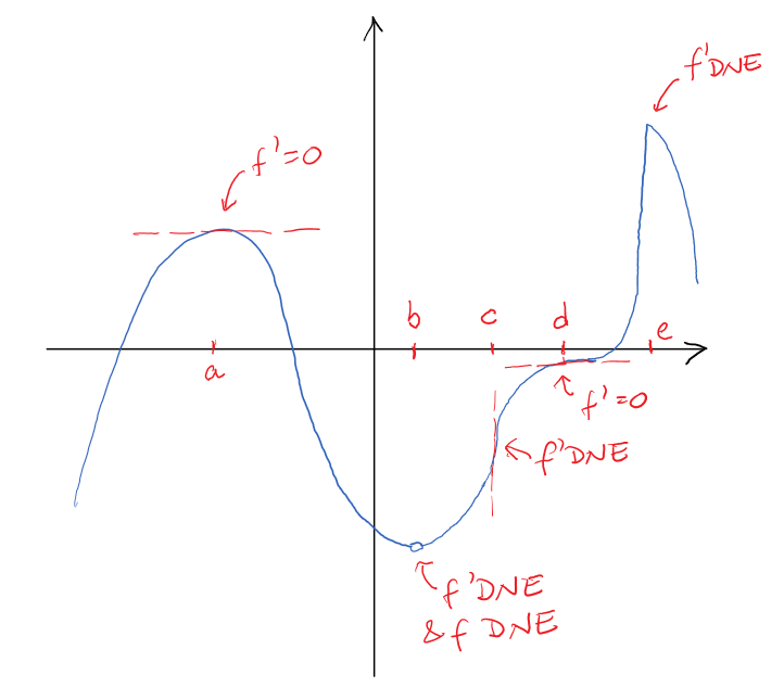 |
[latex]x[/latex] | in domain? | [latex]f'(x)=?[/latex] | critical number? | local extrema? |
| [latex]a[/latex] | yes | [latex]0[/latex] | YES | yes (local max) | |
| [latex]b[/latex] | no | DNE | NO | no | |
| [latex]c[/latex] | yes | DNE | YES | no | |
| [latex]d[/latex] | yes | [latex]0[/latex] | YES | no | |
| [latex]e[/latex] | yes | DNE | YES | yes (local max) |
Fermat's Theorem can be rephrased as follows:
The essential condition for identifying potential local extrema
If a function has a local minimum or maximum at [latex]c[/latex], then [latex]c[/latex] is a critical number of the function.
Therefore, to identify potential local minima and maxima of a function, we must look for them among the critical numbers of the function.
Example 2
Determine the critical numbers of the following function algebraically. Then use a graphing calculator to verify your answer and to identify for each critical number whether the function attains an extrema at that value.
[latex]y=\frac{e^x}{x}[/latex]
Answer: critical numbers of [latex]y[/latex]? verify using graph? visual check for extrema at c.n.?
critical numbers?
critical #s are input values in the domain for which [latex]y'=0[/latex] or undefined [latex]\to[/latex] need the domain,[latex]y'[/latex], and solutions to [latex]y'=0[/latex] or DNE
domain?
domain is all input values that produce an output, i.e., [latex]x=?[/latex] such that [latex]y=\frac{e^x}{x}[/latex] exists
Since [latex]e^x[/latex] is defined for all [latex]x[/latex] and the only other operation is division, which requires that the denominator be non-zero, we have that the only restriction is that [latex]x\neq 0[/latex], i.e.,
domain: [latex](-\infty,0)\cup(0,\infty)[/latex]
[latex]y'=?[/latex]
Since [latex]y[/latex] is a quotient of exp. fn. and linear fn. we have that
[latex]y'=\frac{e^x\cdot x-e^x\cdot 1}{x^2}=\frac{e^x(x-1)}{x^2}[/latex]
[latex]y'=0?[/latex]
Since [latex]y'[/latex] is a quotient, it is equal to zero only when the numerator is zero and the denominator is not zero. Hence
[latex]y'=0\Rightarrow e^x(x-1)=0\Rightarrow e^x=0[/latex] or [latex]x-1=0\Rightarrow x=1[/latex] ([latex]e^x[/latex] is never zero)
Since [latex]x=1[/latex] is in the domain of [latex]y[/latex], [latex]x=1[/latex] is a critical number of [latex]y[/latex].
[latex]y'[/latex] DNE?
Since [latex]y'[/latex] is a quotient of a product of an exponential function with a polynomial, which are defined for all [latex]x[/latex], and the square function (defined for all [latex]x)[/latex]), it is not defined only when its denominator is zero, i.e., when [latex]x^2=0[/latex], i.e., [latex]x=0[/latex], which is not in the domain of [latex]y[/latex] and so it is not a critical number of [latex]y[/latex].
Therefore, [latex]y[/latex] has only one critical number, at [latex]x=1[/latex].
 verification using the graph?
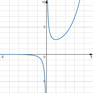
Viewing the function using a graphing calculator (link to graph), it appears that the slope of the graph is zero only at [latex]x=1[/latex] and that the slope exists (no vertical tangents or sharp points) everywhere else on the domain, which excludes [latex]x=0[/latex]. Hence the visual matches our algebraic work.
visual check for extrema at c.n.?
Viewing the graph at [latex]x=1[/latex], the critical number, it appears we have a local minimum there.
Example 3
Determine the critical numbers of the following function algebraically. Then use a graphing calculator to verify your answer and to identify for each critical number whether the function attains an extrema at that value.
[latex]f(x)=\frac{x^2}{x-2}[/latex]
Answer: critical numbers of [latex]f[/latex]? verify using graph? visual check for extrema at c.n.?
critical numbers?
c.n.'s are input values in the domain for which [latex]y'=0[/latex] or undefined [latex]\to[/latex] need the domain,[latex]y'[/latex], and solutions to [latex]f'=0[/latex] or DNE
domain?
domain is all input values that produce an output [latex]\to x=?[/latex] such that [latex]f(x)=\frac{x^2}{x-2}[/latex] exists
Since [latex]x^2[/latex] is defined for all [latex]x[/latex] and the only other operation is division, which requires that the denominator be non-zero, we have that the only restriction is that [latex]x-2\neq 0[/latex], i.e., [latex]x\neq 2[/latex]. Hence,
domain: [latex](-\infty,2)\cup(2,\infty)[/latex]
[latex]f'=?[/latex]
Since [latex]f[/latex] is a quotient of a quadratic and linear function
[latex]f'(x)=\frac{2x\cdot (x-2)-x^2\cdot 1}{(x-2)^2}=\frac{2x^2-4x-x^2}{(x-2)^2}=\frac{x^2-4x}{x-2}=\frac{x(x-4)}{(x-2)^2}[/latex]
[latex]f'=0?[/latex]
Since [latex]f'[/latex] is a quotient, it is equal to zero only when the numerator is zero and the denominator is not zero. Hence
[latex]f'=0\Rightarrow x(x-4)=0\Rightarrow x=0[/latex] or [latex]x-4=0[/latex]=0\Rightarrow x=0,\, 4\leftarrow[/latex] potential c.n.
Since [latex]x=0, 4[/latex] are in the domain of [latex]f[/latex], they are critical numbers of [latex]f[/latex].
[latex]f[/latex] DNE?
Since [latex]f'[/latex] is a rational function, it is not defined only when its denominator is zero, i.e., when [latex](x-2)^2=0[/latex], i.e., [latex]x=2[/latex], which is not in the domain of [latex]f[/latex] and so it is not a critical number of [latex]f[/latex].
Therefore, [latex]y[/latex] has only two critical numbers, at [latex]x=0[/latex] and at [latex]x=4[/latex].
 verification using the graph?
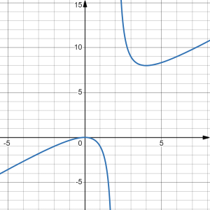
Viewing the function using a graphing calculator (link to graph), it appears that the slope of the graph is zero at [latex]x=0[/latex] and at [latex]x=4[/latex], and that the slope exists (no vertical tangents or sharp points) everywhere else on the domain, which excludes [latex]x=2[/latex]. Hence the visual matches our algebraic work.
visual check for extrema at c.n.?
Viewing the graph, it appears there is a local maximum at [latex]x=0[/latex] and a local minimum at [latex]x=4[/latex].
Let's do one more example, this time with a hand-written solution.
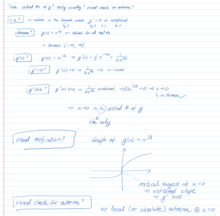
Example 4
Determine the critical numbers of the following function algebraically. Then use a graphing calculator to verify your answer and to identify for each critical number whether the function attains an extrema at that value.
[latex]g(x)=x^{1/3}[/latex]
Answer:
Important note: In what follows it will be of outmost importance that you are able to create sign charts and identify critical numbers almost as easily as doing the multiplication tables. Make sure that you practice both using the exercise set below so that these processes that feel very complex at the beginning of your learning eventually (and very soon) become a routine.
We finish this section by bringing together the Extreme Value Theorem and critical numbers of a function to create a process for identifying the absolute minima and maxima values of a function continuous on a closed interval.
The Closed Interval Method
Given a function [latex]f[/latex] that is continuous on a closed interval [latex][a,b][/latex], we can determine its absolute maxima and minima by performing the following steps:
- Find the value of [latex]f[/latex] at each critical numbers of [latex]f[/latex] on the interval [latex][a,b][/latex].
- Find the value of [latex]f[/latex] at the boundaries of the interval, i.e., [latex]f(a)[/latex] and [latex]f(b)[/latex].
- Compare the values of the function from the first two steps. The largest value represents the absolute maximum and the smallest value represents the absolute minimum.
Example 5
Identify the absolute maxima and minima, if any, of [latex]f\left(x\right)=2x^{3}+3x^{2}-12x+5[/latex] on [latex][-3,0][/latex].
Answer: absolute minima/maxima?
Since [latex]g[/latex] is a polynomial, it is continuous everywhere and so it is continuous on [latex][-3,0][/latex]. By Extreme Value Theorem, [latex]f[/latex] has an absolute maximum and an absolute minimum on [latex][-3,0][/latex]. Using Closed Interval Method, we know that these values will occur either at the critical numbers of [latex]f[/latex] or at the boundaries of the interval.
critical #s?
c.n.'s are values of [latex]x[/latex] in the domain such that [latex]f'(x)=0[/latex] or DNE
domain?
We are looking at the interval [latex][-3,0][/latex] and so the domain is restricted to [latex][-3,0][/latex]
f'(x)=?
[latex]f'(x)=6x^2+6x-12=a(x-x_1)(x-x_2)[/latex]
where [latex]a=6[/latex] and
[latex]x_{1,2}=\frac{-b\pm\sqrt{b^2-4ac}}{2a}=\frac{-6\pm\sqrt{6^2-4\cdot 6\cdot (-12)}}{2\cdot 6}=\frac{6\pm 18}{12}=-2,\ 1[/latex]
Therefore,
[latex]f'(x)=6(x+2)(x-1)[/latex]
f' undef.?
[latex]f'[/latex] is a polynomial so it is never undefined
f'=0?
[latex]f'(x)=0\Rightarrow 6(x-2)(x+1)=0\Rightarrow x=-2, 1[/latex]
Since [latex]x=-2[/latex] is the only one in the given interval [latex][-3,0][/latex], it is the only critical number.
value of [latex]f[/latex] at critical numbers?
[latex]f(-2)=2(-2)^{3}+3(-2)^{2}-12(-2)+5=25[/latex]
value of [latex]f[/latex] at the interval boundaries?
[latex]f(-3)=2(-3)^{3}+3(-3)^{2}-12(-3)+5=14[/latex]
[latex]f(0)=2(0)^{3}+3(0)^{2}-12(0)+5=5[/latex]
Therefore, the absolute maximum value of [latex]f[/latex] is [latex]25[/latex], occurring at the critical number [latex]x=-2[/latex], and the absolute minimum value of [latex]f[/latex] is [latex]5[/latex], occurring at the upper interval boundary [latex]x=0[/latex].
Section Exercises
Work on the following exercises. Discuss your solutions with your peers and/or course instructor.
IC4NITS Exercises 2.7 - Maxima and Minima
