Assume that [latex]y[/latex] is a function of [latex]x[/latex]. Calculate

a. [latex]\frac{d}{dx}\left( y^3 \right)[/latex]

b. [latex]\frac{d}{dx}\left( x^3y^2 \right)[/latex]

c. [latex]\frac{d}{dx}\left( \ln(y) \right)[/latex]

Answer:

a. [latex]\frac{d}{dx}\left( y^3 \right)=?[/latex]

Since [latex]y[/latex] is considered to be a function of [latex]x[/latex], we have that

[latex]y^3=\overbrace{({y(x)})^3}^{composition}=\overbrace{(\text{something involving }x)^3}^{composition}[/latex]

Thus we will need the chain rule since [latex]y^3[/latex] is a power function applied to another (unknown) function of [latex]x[/latex], i.e., a composition of functions.

[latex]\frac{d}{dx}\left( y^3 \right)=\overset{out'}{3y^2}\cdot\overset{in'}{\frac{dy}{dx}}\overset{or}{=}3y^2y'[/latex]

b. [latex]\frac{d}{dx}\left( x^3y^2 \right)=?[/latex]

Let’s analyze the function:

[latex]x^3y^2=\overbrace{x^3\cdot \overbrace{(y(x))^2}^{composition}}^{product}[/latex]

Therefore w need to use the product rule and the chain rule:

[latex]\begin{align*} \frac{d}{dx}\left( x^3y^2 \right) & = \overset{first'}{3x^2}\cdot \overset{second}{\overset{}{y}}+\overset{first}{\overset{}{x^3}}\cdot\overset{second'}{\underset{out'}{\underset{}{2y}}\cdot\underset{in'}{\underset{}{\frac{dy}{dx}}} }\\ & = 3x^2y+2x^3y\frac{dy}{dx} \\\\ &\overset{\text{or}}{=} 3x^2y+2x^3yy' \end{align*}[/latex]

c. [latex]\frac{d}{dx}\left( \ln(y) \right)=?[/latex]

Since [latex]\ln(y)=\ln(y(x))[/latex], this is a composition of functions with no other operations and so we simply apply the chain rule:

[latex]\frac{d}{dx}\left( \ln(y) \right)=\frac{1}{y}\cdot \frac{dy}{dx}=\frac{1}{y}\cdot y'[/latex]

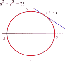
Use implicit differentiation to find the slope of the tangent line to the circle [latex]x^2 + y^2 = 25[/latex] at the point [latex](3, 4)[/latex].

Answer: slope of tangent at [latex](3,4)[/latex]?

The slope of the tangent line will be equal to [latex]\frac{dy}{dx}[/latex] evaluated at the point [latex](3, 4)[/latex].

We differentiate each side of the equation [latex]x^2 + y^2 = 25[/latex] with respect to [latex]x[/latex] and then solve for [latex]y'[/latex]:

[latex]\begin{align*} x^2 + y^2 = 25&\Rightarrow \frac{d}{dx}\left(x^2+y^2\right) = \frac{d}{dx}(25)\\\\ &\Rightarrow 2x+2yy' = 0\\\\ &\Rightarrow 2yy'=-2x\\\\ &\Rightarrow y'=-\frac{x}{y} \end{align*}[/latex]

Therefore, at the point [latex](3,4)[/latex], [latex]y'=-\frac{3}{4}[/latex] and so slope of the tangent line at [latex](3, 4)[/latex] is [latex]0.75[/latex].

Suppose that the wi-fi signal strength [latex]s[/latex] (measured in dBm) and antenna adjustment [latex]a[/latex] (measured in degrees) are related as follows:

[latex]0.5a^{3}s-2a^{2}s^{2}+0.5=0[/latex]

Determine the rate of change in the signal strength when the antenna is adjusted by 5 degrees, giving the signal strength of 1.258 dBm. Interpret your result.

Answer: [latex]ds/da=?[/latex] when [latex]a=5[/latex] and [latex]s=0.792[/latex]; Interpretation?

The given equation cannot be (easily) solved for [latex]s[/latex], so we will use implicit differentiation.

[latex]\begin{align*} 0.5a^{3}s-2a^{2}s^{2}+0.5=0&\Rightarrow \frac{d}{da}(0.5a^{3}s-2a^{2}s^{2}+0.5)=\frac{d}{da}\left(0\right)\\\\ &\Rightarrow 1.5a^2\cdot s+0.5a^3\cdot\frac{ds}{da}-4as^2-2a^2\cdot \left(2s\cdot \frac{ds}{da}\right)+0=0\\\\ &\Rightarrow 1.5a^2s+0.5a^3\cdot\frac{ds}{da}-4as^2-4a^2s\cdot \frac{ds}{da}=0\\\\ &\Rightarrow \frac{ds}{da}\left(0.5a^3-4a^2s\right)=4as^2-1.5a^2s\\\\ &\Rightarrow \frac{ds}{da}=\frac{4as^2-1.5a^2s}{0.5a^3-4a^2s} \end{align*}[/latex]

At [latex]a=5[/latex] and [latex]s=1.258[/latex] we have

[latex]\dfrac{ds}{da}=\dfrac{4\cdot 5\cdot 1.258^2-1.5\cdot 5^2\cdot 1.258^2}{0.5\cdot 5^3-4\cdot 5^2\cdot 1.258}\approx 0.245[/latex]

and so at 5 degrees in antenna adjustment when the signal strength is 1.258 dBm, the signal strength is increasing by approximately 0.245 dBm per degree in antenna adjustment.

How fast is the surface of a cube increasing if its width is increasing at the rate of 2 cm/min when the width of the cube is 15 cm?

Answer: [latex]\dfrac{dS}{dt}=?[/latex] where [latex]S[/latex] is the surface area (cm²) of a cube and [latex]t[/latex] is time (min), given a width and rate of change in width

Note that we are looking for a rate of change in the surface area and we are given information about the rate of change in width. So we first consider what we know about the relationship between the surface area of the cube and its width. Recalling our knowledge about basic geometry, we know that if [latex]w[/latex] is the width of the cube, then:

[latex]S=6w^2[/latex]

We can now use implicit differentiation to determine the rate of change in the surface area in relation to time by taking the derivative of both sides of that equation with respect to [latex]t[/latex]:

[latex]\begin{align*} S=w^3&\Rightarrow\frac{d}{dt}\left( S \right)= \frac{d}{dt}\left(6w^2 \right)\\ &\Rightarrow\frac{dS}{dt}= 12w\frac{dw}{dt} \end{align*}[/latex]

Substituting in the values we know for [latex]w[/latex] and [latex]\frac{dw}{dt}[/latex], we have

[latex]\frac{dS}{dt}=12(15)(2)=360[/latex]

So the surface area of the cube is increasing by approximately 360 square cm per min when the width is 15 miles and increasing by 2 cm per minute.

A company is using an AI-based weekly predictor of the company’s network usage. Its network analysts ran a test that measured the accuracy [latex]A[/latex] of the predictor (as a percent of accuracy) in relation to the number of data points [latex]n[/latex] used by the predictor. They modeled the predictor’s accuracy using

[latex]A(n)=2.55\sqrt{n+250})+40.3[/latex]

If the number of data points is decreasing by 150 per test when the number of data points is 3000, what is the rate of change in the accuracy of the predictor per test? Express your result as a percent, rounded to two decimals. Briefly explain the meaning of your result in the context of the question.

Answer: [latex]\dfrac{dA}{dT}=?[/latex] where [latex]T[/latex] is the number of tests

We are given information about the rate of change in the number of data points in relation to the number of tests and so we can apply implicit differentiation to the relationship between predictor accuracy [latex]A[/latex] and number of data points [latex]n[/latex] to find the rate of change in the accuracy in relation to the number of tests run. In this case we will view both the accuracy and the number of data points as functions of the number of tests (even though the accuracy is also a function of number of data points):

[latex]\begin{align*} A=2.55\sqrt{n+250}+40.3&\Rightarrow A=2.55(n+250)^{1/2}+40.3\\ &\Rightarrow \frac{d}{dT}(A) = \frac{d}{dT}\overset{sum}{\left(\overset{composition}{2.55(n+250)^{1/2}}+\overset{constant}{40.3}\right)} \\ &\Rightarrow \frac{dA}{dT} = 2.55\cdot \frac{1}{2}\left(n+250\right)^{-1/2}\cdot\left(\frac{dn}{dT}+0\right)+0 \\ &\Rightarrow \frac{dA}{dT} = 2.55\cdot \frac{1}{2}\left(n+250\right)^{-1/2}\cdot\frac{dn}{dT} \end{align*}[/latex]

Using the given information, we know the number of data points is decreasing by 150 per test when there are 3000 points, so

[latex]\frac{dA}{dT} = 2.55\cdot \frac{1}{2}\left(3000+250\right)^{-1/2}\cdot(-150)\approx-3.35[/latex]

Therefore, when there are 3000 points and the number of data points is decreasing by 150 per test, the predictor accuracy is decreasing by approximately 3.35% per test.