Installing Fiji (A.K.A. ImageJ2):

In the case of seeing the error in the first image, find the Fiji file, right click, and select ‘Open.’ The message in the second image should appear instead. Click ‘Open’ and the error will resolve. If you downloaded Fiji from the correct site, there should be no concerns opening the file, even if it is unverified.

2. If Fiji warns you that the file needs to be moved from the downloads folder, we recommend moving Fiji onto the desktop or in the applications folder. It is possible that keeping Fiji in the downloads folder will not let it update properly, or hinder the installation of MosaicSuite.

Installing and using the MosaicSuite for ImageJ to track particles

The MosaicSuite is a bundle of ImageJ extensions (“plugins”) developed by Dr. Ivo Sbalzarini at the Center for Systems Biology Dresden in Germany. These plugins allow performing a number of advanced image analysis procedures.

In this lab, we will make use of one of the plugins in the MosaicSuite called Particle Tracker 2D/3D.

Installation.

To install MosaicSuite, follow the instructions given on the Mosaic website: http://mosaic.mpi-cbg.de/?q=downloads/imageJ. The following is the basic setup, accompanied by a video recorded on macOS Fiji:

1. Open Fiji.
2. Go to Help > Update…
3. Let Fiji update if required. This may take a few minutes.
4. Click Manage Update Sites.
5. Search ‘Mosaic’ or scroll until you find ‘MOSAIC ToolSuite.’
6. Check ‘MOSAIC ToolSuite,’ then hit Apply and Close.
7. Click Apply Changes and let the installer run.
8. Restart Fiji.
9. You can now access MosaicSuite tools in the plugin menu, under ‘Mosaic.’

Tracking particles.

We are going to practice tracking particles using a very simple movie showing the simulated Brownian motion of five different particles (this movie was generated with NetLogo). As there is no noise in this movie, and the particles are always clearly visible, the tracking in this case is easy.

• Start by downloading the movie, called “BrownianMotionSimulation.avi” from Avenue to Learn, and open it with Fiji (File -> Open). When prompted, chose “Convert to Grayscale”. Do not use a virtual stack. The movie should show five perfectly white particles on a perfectly black background.
• To help ImageJ track particles, we will need an estimate of the radius of the particles, in pixels. Use the “Measure” or “Plot Profile” tool, both found in the “Analyze” drop-down menu in Fiji, to get an estimate of this parameter.

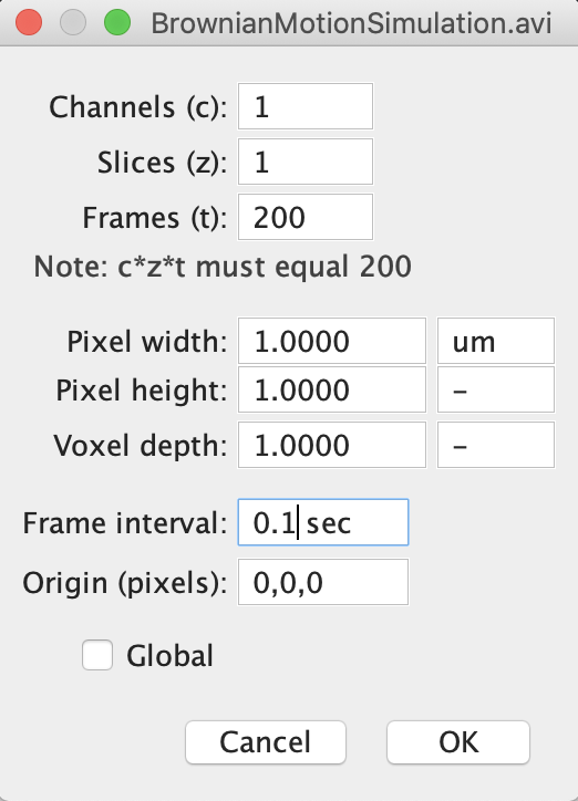
• Next, go to Image -> Properties in order to enter information about the movie which will be needed later to calculate the diffusion coefficient of the particles.
  • By default, ImageJ considers that a stack of images are images taken in different focal planes. To indicate that instead your stack of image is a movie (with each image acquired in the same place but at a different time), set the number of slices to 1 (meaning that all images are in the same focal plane), and set the number of frames to the actual number of frames in the movie (i.e. you have to exchange the values for slice and frame).
  • In that same properties window, enter the correct frame interval (0.1 s), and the correct pixel width in micron (1 um, where “um” stands for “micron”).
  • The properties window should now look like this:
• We are now ready to use the tracking plug-in to detect the position of the beads in all the images in the video.
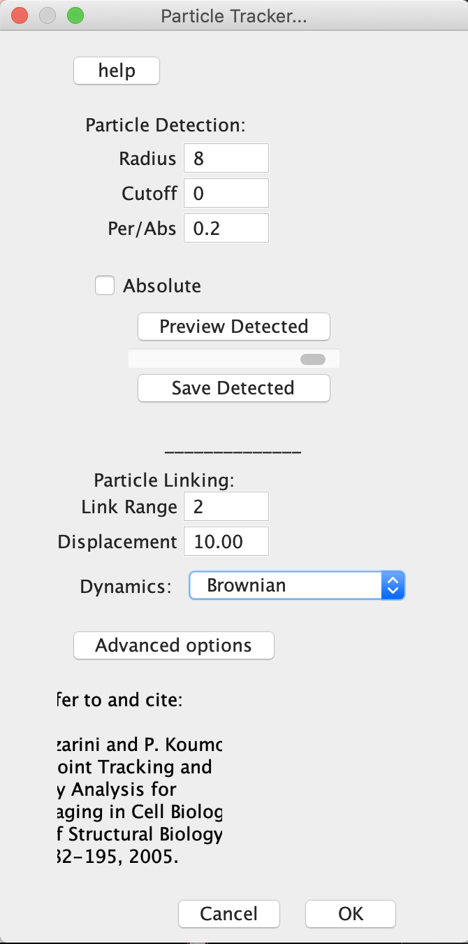
  • Chose: Plugins -> Mosaic -> Particle tracker 2D/3D. A Particle Tracker window opens, which is divided in two parts: The upper part is devoted to particle detection (the identification and location of all particles in all images), and the lower part to particle linking (the building of trajectories for each individual particles throughout the whole movie).

• • To help the identification of the beads, you will need to set three parameters:
    • “Radius” is the radius of the particles in pixels. It should be set to a value slightly larger than that you estimated.
    • “Cutoff” is a threshold value that determines how selective the program will be in deciding that a particle is really a particle. Start with the cutoff value at “0” (all detected particles are accepted), and increase by 1 or 2 units if you find that objects that are not particles are detected. Repeat as necessary.
    • “Percentile” determines how hard the program is looking for particles. Start with a value of 0.1%, which means that all spots with an intensity within 0.1% of the intensity of the brightest pixel in the image will be considered as possibly belonging to a particle. If not enough particles are being detected, try increasing this value, and vice versa.
    • Press “Preview Detected” and check that all the particles that you see in the first image are correctly detected (as indicated by a single red circle). If you are not happy, change the particle detection parameters until the detection is optimal. You should check the quality of the detection for several images throughout the movie by moving the slider and pressing “Preview detected” again. For this simple movie without background noise, this should be fairly easy.
  • Once you are happy with the detection, you can move on to the “Particle Linking” part of the algorithm, which builds particle trajectories.
    • Set the field value “Link Range” to 1. This parameter determines for how many frame interval a particle can “disappear” before it is considered truly lost. In this movie, particle should never be lost, but for a noisier movie the value of Link Range should be increased.
    • The value of the field “Displacement” should be set to at least twice the average displacement of a particle (in pixel) between two frames. This parameter determines the “search radius” used to find a given particle in the next frame.
    • Click Ok. After some time (this step may take some time), a new window called “Results” will appear in which you can see how many trajectories have been found.
    • To visualize these trajectories, press “Visualize all trajectories”, which should open a new window called “All Trajectories Visual (V)”. Drag the cursor at the bottom of this window to navigate through the movie and see the detected trajectories, each of which will be drawn with a different color.
    • If you are happy with the trajectories, you can save the corresponding particle positions in a table (“All trajectories to table”).
  • Our main goal in this lab is to obtain the diffusion coefficient of the particles, D, from the detected trajectories. We can do this easily with the particle tracker by plotting their mean-squared displacement (MSD) as a function of time.
  • Select a particular trajectory by clicking on it in the “All Trajectories Visual (V)”. A yellow box will appear around that trajectory once if it has been properly selected.
  • 
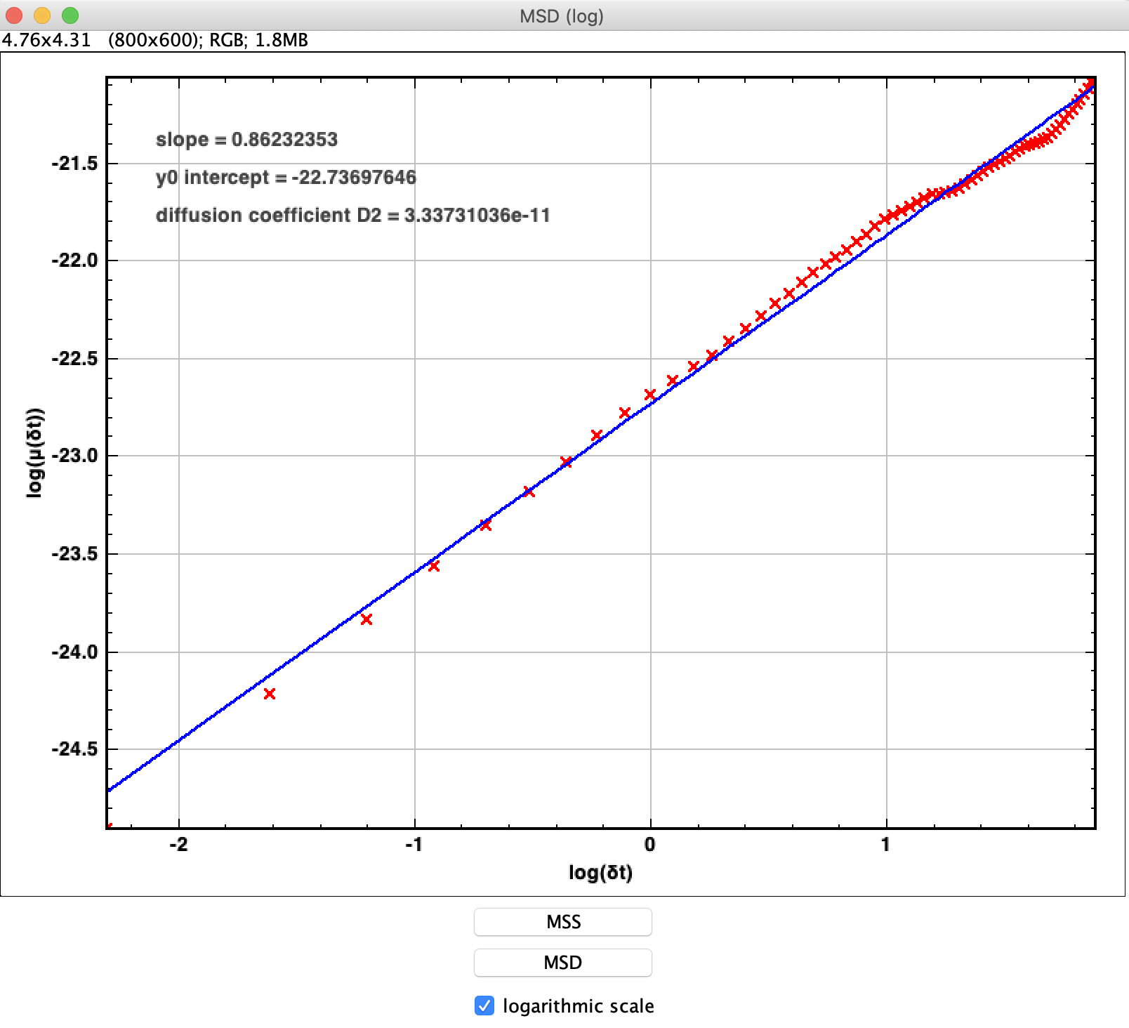
  • Once a trajectory is properly selected, press “MSS/MSD plots” in the “Results” window, then press “MSD” at the bottom of the newly created window, in order to obtain a log-log plot of the particle MSD as a function of time. You should get a plot which looks like this:
  • The slope of the MSD (on a linear scale) should be equal to 4D. This means that, on a log-log scale, the y-intercept of the MSD is equal to . The tracking plugin automatically fits the curve for you, and returns both the value of the y-intercept and the value of , in units of m²/s (but only if you have properly entered the information about pixel width and frame interval!!!).
  • If you want to plot and analyze the MSD yourself, press “MSS/MSD to Table” in the “Results” window.