Smoothing Data to Remove Noise

Data from mechanical systems usually changes fairly slowly compared to electrical systems and we can often define a characteristic time or frequency and ignore changes in the data that happen any faster. Some sort of time averaging over multiple samples will smooth out the sample to sample variations, reducing the noise at frequencies near the sampling frequency and providing a better estimate of actual values. Often we must make immediate decisions based on the data we have available to date. The recent COVID-19 pandemic provides a stark example of the need to interpret limited data in as timely a fashion as possible. We have all been watching this data closely and need the skills to assess it critically. Different control choices made in the spring have so far led to significantly different outcomes.

Notice how important it is to use the right approach to smoothing when interpreting the data. Averaging over larger sample sizes also reduces the noise in the data.

An Exponential Smoothing example is provided in the RWS-Notes/Code-Arduino/Learning Sequence SAMD/ S1.3_New_Tab_and_Smoothing sketch (Arduino S1.3)

Post-Processing of Time Series Data

If you wait until after a full time series data set is collected, you can base your estimates for the actual value at a particular time on data from both before and after that time. Knowing something about the future allows better estimates of the present. Processing offline reduces the pressure to complete calculations quickly, allowing for more sophisticated techniques. However, it doesn’t allow you to take any action in the present.

Any technique that can be applied in real time can also be applied in post-processing. This can be really useful for testing different estimating approaches to processing the same data.

Real Time Processing of Time Series Data

Improving your estimates from time series data during acquisition is essential for acting immediately on those estimates to control the system being measured, however it comes with two key limitations:

• The current estimate for a measured quantity can only depend on the current measurement and other measurements made in the past.
• The current estimate must be calculated quickly enough to be useful in real time, usually before the next measurement is made.

Exponential Smoothing (Python 4.2) is easier to implement on a microcontroller (Arduino S1.3) than Moving Averages (Python 4.1). Smoothing provide some influence of the long time history of your data to make an estimate in the present, without needing to store all the past values in an array.

Taking Derivatives of Measured Data

Numerical differentiation is simple in concept, but those small differences in will amplify any noise that was there in either the time base, or in the measured values. This video (7:26) provides the basics of differentiating position to get velocity and acceleration estimates.

These two videos will help understand the sources of the differentiation noise we see in the lab and test out strategies for reducing it. By simulating the measurement, smoothing, and differentiation processes in software (Python 4.5), we can better understand the problems they generate. (video 22:02 & 11:46)

This simple differencing approach requires data for only two points in time, reducing the computational and storage overhead for limited capacity microcontrollers. More complex techniques for estimating derivatives will be covered in detail in your numerical analysis courses, and will require more history data to be stored. A pencil and paper uncertainty analysis supports the numerical results we go above (video 9:54).

Integrating Measured Data Over Time

Integration over time will provide not just instantaneous measurements, but their accumulated results over time. Integrating a flow rate will give the total volume of fluid delivered, perhaps the total litres of air breathed in during a single or multiple breaths. Integrating a velocity will give total distance travelled.

Use a global or static variable to accumulate your integral so that the total is remembered between loop calls. Each time step will add for the period just finished, which could be calculated as , or even just to yield the same long term integration.

Although integration is insensitive to noise because the highs and the lows will average out over time, any bias in the measurement will accumulate with every step in the integration. This may not be an issue if you are totalling a flow, but bias errors in measurements will make integrations of oscillating values drift off over time, so you may want to reset the total to zero when you reach some landmark in your measurement.  For example: A long time integration of flow in and out of your lungs should be close to zero if everything that went in was breathed out, but a positive bias in the measurement may give an integration suggesting you have reached hundreds of litres of air in your lungs over time, even if the estimates for each breath a reasonably accurate.

This video (6:03) explains how to numerically integrate a signal like an acceleration and the sample code implements the calculation on the Arduino, using an ideal cosine function in place of an accelerometer measurement.

Integration is essentially just addition, and fairly accurate as long as the time steps are short. Any bias error in the measured values will build up as a large drift over time. What effect will noise have?

Tracking Detailed Time Series Data

More detailed analysis of your data will require storage of more than a couple of data points. Storing a full set of data on your microcontroller will quickly overwhelm its storage capacity, so you will need to keep those limitations in mind to eliminate the oldest history data as you go along. The simplest approach is to transfer the history data to your computer and look at it later.

All measurements have a time frame for when the measurement was made, even if the measurement was made only once:

  “The freezer temperature is -18C. I know because I measured it this morning.”

tells us that the freezer was at -18C this morning, but it doesn’t tell us what has happened since then. The time series might look like this:

2015-11-11 11:11:11  -18.0

The time stamp suggests that I know to within seconds just when the measurement was completed. The .0 in 18.0 suggests that my uncertainty in the temperature is in tenths of a degree. Measuring more often will let me see how the temperature is changing with time:

2015-11-11 11:11:11  -18.0
2015-11-11 11:21:11  -17.8
2015-11-11 11:31:11  -17.6
2015-11-11 11:41:11  -17.7
2015-11-11 11:51:11  -17.3
2015-11-11 12:01:11  -16.8
2015-11-11 12:11:11  -18.5
2015-11-11 12:21:11  -18.3
2015-11-11 12:31:11  -18.4
2015-11-11 12:41:11  -18.1

It looks like the freezer warmed up for a while until it got above -17C around noon when the thermostat kicked in, cooled it right back down, then it started getting warmer again. It will probably get back up to 17C around 13:30 if everything else remains the same. We know a lot more about this system because we know what time the measurements were taken. If we just knew the values:

-16.8, -17.3, -17.6, -17.7, -17.8, -18.0, -18.1, -18.3, -18.4, -18.5

it would tell us a lot less about the behaviour of the freezer.

Every measurement needs a timestamp. You can use the same timestamp for multiple measurements made at close to the same time

2015-11-11 11:11  -18.0  -27.3  26.5

might be a line telling me that at 11:11 the air in the freezer was -18.0C while the refrigerant in the cooling coils was at -27.3C and the room temperature was 26.5C. Obviously some column headers will make it easier to understand the data:

Date       Time   Frzr   Coolnt Room
2015-11-11 11:11  -18.0  -27.3  26.5

The ISO Standard for Dates is YYYY-MM-DD so be sure to use it! Use HH:MM:SS.ssssss for time of day with as many ssss as needed to resolve your timescale. When you don’t know the date or time, just record your timebase in seconds, milliseconds, microseconds as appropriate to the application.

Store Your Time Series in CSV Files to make your life easier

We  will often be looking at data recorded as a function of time, that would be easily organized into a table with a row for each time and a column for each different measurement. These files might be copied and pasted from the Serial Monitor to your computer, or stored on an SD card directly on your microcontroller if one is available. To move data back and forth between different programs we will use files of Comma Separated Values (CSV) where every line represents a row in the table like this:

Time [us], analog0, V0, another thing
12345, 359, 1.75, 122.34
23456, 365, 1.89,  222.56
...
12345, 359, 1.75, 122.34

It’s easy to write data like this with Serial.print() from the Arduino to the serial monitor window. From there you can select it and copy it with the usual ^A ^C, etc. keys or the mouse.

In Windows paste the data into Notepad and save as e.g. “test.csv”

On a Mac open TextEdit. Go to preferences and choose New Document / Plain Text instead of Rich Text and under Open and Save uncheck the Add “.txt” extension to plain text files. Then open a new document, paste your data, and save as e.g. “test.csv” so you can open it later in whatever program you want.

If you store your data this way it will be easy to load it into Excel later just by double clicking. You can also load it directly into Matlab or read it easily in Python.

Pasting CSV Data Direct to Excel

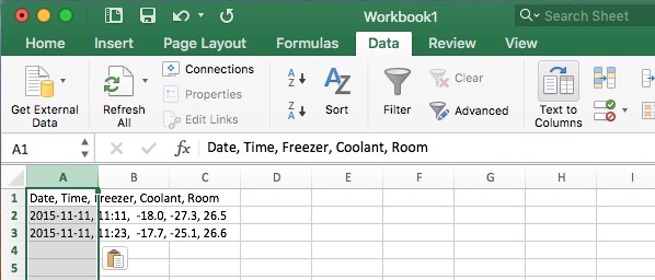
Date, Time, Freezer, Coolant, Room
2015-11-11, 11:11,  -18.0, -27.3, 26.5
2015-11-11, 11:23,  -17.7, -25.1, 26.6
2015-11-11, 11:25,  -17.7, -24.2, 26.5
2015-11-11, 11:29,  -17.3, -21.1, 23.1

Copy the first three lines of that text and paste it into Excel. Use Data/Text to Columns to separate the parts.

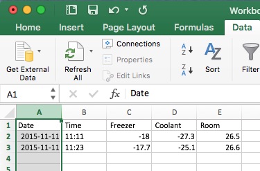
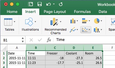
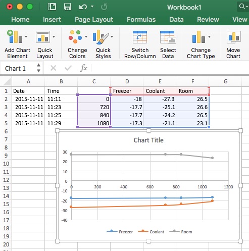
Highlight the columns as shown and insert a chart.

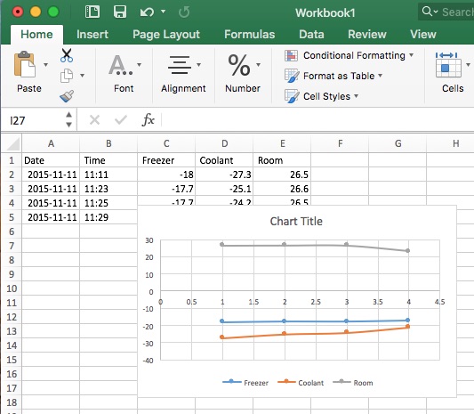
Even if you used a scatter plot, Excel may have a hard time figuring out what to do with those textual time stamps, so a plain number would work better. The top row label needs to be blank to get Excel to treat it as the X axis value.

Date, Time, , Freezer, Coolant, Room
2015-11-11, 11:11, 0,  -18.0, -27.3, 26.5
2015-11-11, 11:23, 720,  -17.7, -25.1, 26.6
2015-11-11, 11:25, 840,  -17.7, -24.2, 26.5
2015-11-11, 11:29, 1080,  -17.3, -21.1, 23.1

Collect an Array of Data for Immediate Batch Processing

Larger microcontroller storage spaces will allow you to store multiple values and the corresponding time stamps in arrays. You can then process that data in quasi-real time right on the microcontroller. For example, you might accumulate 1024 data points at uniform time intervals, then use a Finite Fourier Transform (FFT) to extract the recent dominant frequencies to see if a vibration problem is developing in your equipment. FFT is sometimes used as an abbreviation for FAST Fourier Transform, and good algorithms will allow you to do these calculations many times per second. 1024 floats, requires 4096 bytes (4kB) of memory, more than you could manage on an UNO or equivalent, but well within the capacity of most 32 bit microcontrollers like the SAMD M0 on the Itsy Bitsy.

Maintain a Continuous Data Buffer Array

Knowing a single current value tells you nothing about rates of change, and even carrying along an additional value from the past iteration provides limited information. Sometimes it is valuable to have a full sequence of values over time to provide a bigger picture. There are at least two approaches we could take:

• Keep a list in order from oldest to newest as the array index goes from 0 to NPTS-1. Every time through the loop, move all the values one step up the list and add a new value at the end. While this is intuitive and always keeps the list in order, the shuffling all the data up one step requires many operations every time you get a new data value.
• Keep track of where you are in the list with an index, so you know where to put the latest value and there’s no need to shuffle. Move the index back to zero when you get to the end of the  array and start again. This is much more efficient while you collect the data, but requires a little more code to keep track of where the list begins, so you can start in the middle with the oldest value and wrap around to the newest.

This video (10:57) shows both approaches and adds a few features to better keep track of time. Full arrays of data like this are especially useful for processing with FFTs to extract frequency information from your signals.

The position you just wrote on will always contain the newest values and the position right after it will always contain the oldest. Writing a new value into this fixed size buffer overwrites the oldest value, essentially throwing it away. Modulo arithmetic for the array indices makes it easy to process the data in place, with references relative to the position you are about to write. An array like this is often referred to as a ring buffer because of the way it loops back on itself.