Matin Yousefabadi
EEG Analysis in R: An Educational Guide
Introduction to electroencephalography (EEG)
Electroencephalography, or EEG, is a non-invasive neuroimaging technique that measures and records the electrical activity of the brain. It involves placing electrodes on the scalp to detect the voltage fluctuations resulting from ionic current within the neurons of the brain. EEG provides a real-time representation of brain activity and is widely used in computational neuroscience to study neural processes and understand brain function.
In computational neuroscience, EEG data is analyzed using advanced algorithms and mathematical models to extract valuable information about cognitive processes, sensory perception, and various neurological disorders. Researchers use EEG to investigate patterns of neural activity, brain connectivity, and the temporal dynamics of information processing. The versatility and temporal precision of EEG make it a valuable tool for studying brain function and contributing to our understanding of the complex interplay of neurons in the human brain.
EEG Frequency Bands
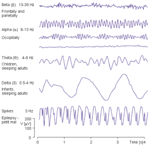
EEG signals are characterized by different frequency bands that reflect the underlying neural activity. The frequency bands are defined based on the frequency range of the EEG signal, and each band is associated with a specific type of brain activity. The frequency bands are as follows:
- Delta (δ) waves (0.5-4 Hz):
- Delta waves are prominent during deep sleep and indicate the brain’s slowest oscillations.
- Abnormalities in delta activity may be linked to certain sleep disorders and neurological conditions.
- Theta (θ) waves (4-8 Hz):
- Theta activity is observed during drowsiness, meditation, and REM (rapid eye movement) sleep.
- Increased theta waves are associated with creative thinking and memory consolidation.
- Alpha (α) waves (8-12 Hz):
- Predominant during relaxed wakefulness, with eyes closed.
- Alpha waves are linked to a calm and alert mental state.
- Beta (β) waves (12-30 Hz):
- Present during active wakefulness and cognitive tasks.
- Higher beta frequencies are associated with increased mental alertness and concentration.
- Gamma (γ) waves (30-100 Hz):
- Associated with high-level cognitive processes, perception, and problem-solving.
- Abnormal gamma activity may be linked to certain neurological disorders.
Studying the interplay of these EEG bands provides valuable information about brain function, aiding researchers and clinicians in understanding cognitive processes, diagnosing disorders, and developing therapeutic interventions. EEG data analysis allows for the exploration of brain dynamics and can unlock new insights into the complexities of the human mind.
EEG Channels and Electrode Placement
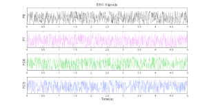
In EEG (Electroencephalography) data, channels refer to the specific locations on the scalp where electrodes are placed to record electrical activity produced by the brain. These electrodes are part of an EEG cap or array. Each channel corresponds to a unique electrode, and the signals collected from these channels collectively provide a comprehensive view of brain activity.
The placement of channels is crucial for capturing signals from different regions of the brain. Common international standards, such as the 10-20 system, are used to define the locations of these channels. The system is named after the fact that the distance between adjacent electrodes is approximately 20% of the total front-to-back or right-to-left distance of the skull, depending on the region. Each channel records the voltage fluctuations over time, reflecting the electrical activity of the neurons in the underlying brain region. Analyzing EEG data from multiple channels allows researchers and clinicians to examine the spatial distribution of brain activity and identify patterns associated with various cognitive states, disorders, or specific tasks.
EEG data analysis in R
In this section, we focus on analyzing EEG data using R. Even though EEG data analysis can be performed using both MATLAB and R, and the choice between the two often depends on the preferences of the researcher, the availability of specific toolboxes or packages, and the nature of the analysis, MATLAB is a more popular choice for EEG data analysis due to its wide range of packages for EEG data analysis.
Key R Packages:
There are various packages and tools to preprocess, visualize, and extract meaningful insights from the EEG recordings. Below is a brief overview of the some typical steps involved in EEG data analysis using R:
eegkit: A package for importing and preprocessing EEG data in R.eegUtils: A package for performing basic EEG preprocessing and plotting of EEG data.ERP: A package for analyzing, identifying and extracting event-related potentials (ERPs) related to specific stimuli or events in R.
Key Software:
EEGLAB: A MATLAB toolbox for processing and analyzing EEG data. It includes a variety of functions for importing, preprocessing, visualizing, and analyzing EEG data. EEGLAB also provides a graphical user interface (GUI) for performing EEG data analysis.FieldTrip: A MATLAB toolbox for analyzing EEG and MEG data. It includes algorithms for simple and advanced analysis of MEG and EEG data, such as time-frequency analysis, source reconstruction using dipoles, distributed sources, and beamformers, connectivity analysis, and non-parametric statistical testing.Brainstorm: A MATLAB toolbox dedicated to the analysis of brain recordings: MEG, EEG, fNIRS, ECoG, depth electrodes and multiunit electrophysiology
EEG Processing and Statistical Analysis in R
EEG Preprocessing
This process aims to remove noise, artifacts, and other unwanted elements while preserving the integrity of the neural signals. Effective preprocessing ensures reliable results in subsequent analyses, focusing on genuine neural activity. Here are key steps involved in EEG data preprocessing:
- Filtering:
- Remove unwanted noise and artifacts by applying filters. Low-pass filters eliminate high-frequency noise, while high-pass filters remove slow drifts.
- Notch filters can be used to eliminate specific frequencies, such as power line interference.
- Artifact Removal:
- Identify and remove artifacts caused by eye movements, muscle activity, or external interference.
- Techniques like Independent Component Analysis (ICA) can help separate and eliminate artifacts from the EEG signal.
- Segmentation:
- Divide the continuous EEG signal into shorter segments, making it easier to analyze specific events or tasks.
- Segmentation allows researchers to focus on epochs of interest, such as stimulus presentation or motor responses.
- Baseline Correction:
- Adjust the EEG signal to have a consistent baseline, often by subtracting the average signal over a specific pre-stimulus period.
- Baseline correction helps in comparing the relative changes in EEG amplitudes during different experimental conditions.
- Referencing:
- Choose an appropriate reference for the EEG data. Common references include average reference or linked mastoids.
- Referencing ensures that the recorded signals reflect the activity relative to a defined point.
- Interpolation:
- Handle missing or bad channels by interpolating their values based on surrounding electrode information.
- This step maintains the spatial integrity of the EEG data.
- Normalization:
- Normalize EEG amplitudes if necessary, facilitating comparisons across different subjects or experimental conditions.
By implementing these preprocessing steps, researchers can enhance the quality of EEG data, reduce noise, and improve the accuracy of subsequent analyses, leading to more reliable insights into brain function and cognition.
Statistical Analysis of EEG Data
Statistical analysis of EEG (Electroencephalography) data is crucial for drawing meaningful conclusions from experimental results. EEG experiments often involve comparing conditions, groups, or time points to uncover patterns of brain activity associated with specific cognitive processes or experimental manipulations. Here’s an overview of key considerations and methods in the statistical analysis of EEG data:
- Descriptive Statistics:
- Utilize measures such as mean, median, and standard deviation to provide a summary of the central tendency and variability of EEG signals.
- Descriptive statistics offer a preliminary understanding of the data’s characteristics.
- Inferential Statistics:
- Apply inferential statistics to make predictions or inferences about the larger population based on the observed EEG data.
- Common tests include t-tests, ANOVA, and regression analysis to assess the significance of differences between conditions or groups.
- Time-Frequency Analysis:
- Employ techniques like Fast Fourier Transform (FFT) to analyze the frequency content of EEG signals over time.
- Time-frequency analysis provides insights into dynamic changes in brain activity associated with different tasks or stimuli.
- Event-Related Potentials (ERPs):
- Extract and analyze ERPs to examine neural responses associated with specific events or stimuli.
- Statistical methods help identify significant ERP components and differences between experimental conditions.
- Clustering and Classification:
- Use clustering algorithms to group EEG patterns, revealing hidden structures in the data.
- Classification methods, such as machine learning algorithms, can discriminate between different cognitive states or conditions.
- Correlation Analysis:
- Explore relationships between EEG features and behavioral or clinical variables.
- Correlation analysis helps identify associations that contribute to a comprehensive understanding of brain-behavior relationships.
- Multiple Comparison Correction:
- Implement correction methods, such as Bonferroni or False Discovery Rate (FDR), to address the issue of inflated Type I error rates when conducting multiple statistical tests.
- Topographic Mapping:
- Create topographic maps to visualize spatial distributions of EEG activity.
- Statistical analyses can highlight significant differences in brain regions during various experimental conditions.
By employing these statistical approaches, researchers can draw robust conclusions from EEG data, uncover patterns, and elucidate the neurophysiological mechanisms underlying cognitive processes or clinical conditions.
Using eegkit for EEG Data Analysis in R
# Install eegkit package
install.packages("eegkit")
# Load eegkit package
library(eegkit)
# Load EEG data
data("eegdata")
# View the first 5 rows of the data
head(eegdata)eegsmooth Smooths single- or multi-channel electroencephalography (EEG) with respect to space and/or time
- Example: Smoothing the data with respect to time
## get "PZ" electrode of "c" subjects
idx <- which(eegdata$channel=="PZ" & eegdata$group=="c")
eegdata1 <- eegdata[idx,]
## temporal smoothing eegmod <- eegsmooth(eegdata1$voltage,time=eegdata1$time) ## define data for prediction time <- seq(min(eegdata1$time),max(eegdata1$time),length.out=100) yhat <- predict(eegmod,newdata=time,se.fit=TRUE) ## plot results using eegtime eegtime(time*1000/255,yhat$fit,voltageSE=yhat$se.fit,ylim=c(-4,4),main="Pz")
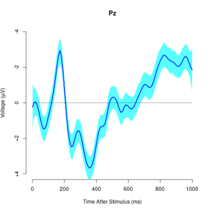 `eegtime` Creates plot of single-channel electroencephalography (EEG) time course with optional confidence
interval. User can control the plot orientation, line types, line colors, etc.
Example: Plotting a single channel
`eegtime` Creates plot of single-channel electroencephalography (EEG) time course with optional confidence
interval. User can control the plot orientation, line types, line colors, etc.


Example: Plotting a single channel
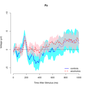
## get "PZ" electrode from "eegdata" data
idx <- which(eegdata$channel=="PZ")
eegdata2 <- eegdata[idx,]

## get average and standard error (note se=sd/sqrt(n))
eegmean <- tapply(eegdata2$voltage,list(eegdata2$time,eegdata2$group),mean)
eegse <- tapply(eegdata2$voltage,list(eegdata2$time,eegdata2$group),sd)/sqrt(50)

## plot results with legend
tseq <- seq(0,1000,length.out=256)
eegtime(tseq,eegmean[,2],voltageSE=eegse[,2],ylim=c(-10,6),main="Pz")
eegtime(tseq,eegmean[,1],vlty=2,vcol="red",voltageSE=eegse[,1],scol="pink",add=TRUE)
legend("bottomright",c("controls","alcoholics"),lty=c(1,2),
       lwd=c(2,2),col=c("blue","red"),bty="n")
Further Reading and References:
- The online EEGLAB workshop provides a tutorial on EEG data analysis in MATLAB.
- More detailed information on EEG data analysis in R can be found in the eegkit documentation.
- For more information on EEG data analysis in Python, check out the MNE documentation.
- For more information on EEG data analysis in MATLAB, check out the EEGLAB documentation.
An example of an statistical EEG Study: Group Differences in Voltage Levels
In a study examining EEG recordings, data from 10 alcoholics and 10 control subjects were collected during a 10-second experiment. The dataset comprises four columns: “ID,” “Group,” “Timestep,” and “Voltage.”
Exploratory Analysis in R
- Load the EEG dataset using the
read.csv()command in R. - In the dataset,
Groupis a factor with two levels:ControlandAlcohol.
Statistical Analysis in R
Perform the following analyses using the loaded data:
- EEG Plotting:
- Create a line plot to visualize the EEG voltage over time for the participant with ID 1.
- Descriptive Statistics:
- Calculate descriptive statistics (mean, standard deviation, etc.) for the “Voltage” column within each group (alcoholics and control subjects).
- T-Test:
- Perform an independent samples t-test to assess if there is a significant difference in mean voltage values between alcoholics and control subjects. Make inferences based on the results.
- ANOVA Analysis:
- Conduct an analysis of variance (ANOVA) to evaluate whether there are significant differences in mean voltage values among the groups. Make inferences based on the results.
This study aims to explore and statistically analyze the EEG data to determine if there are discernible differences in voltage levels between alcoholics and control subjects. The combination of exploratory visualization and statistical tests provides a comprehensive understanding of the EEG patterns and potential group distinctions.
Files to Download:
Answer Key
# Read the CSV file
## Note: this is a simplified simulated EEG data from 10 alcoholic and 10 control subjects participating in a 10 second experiment
## the voltage is recorded with dt=0.01s
data <- read.csv("eeg.csv")
# Plot EEG of one participant
participant_id <- 1 # Change this to the desired participant ID
participant_data <- data[data$ID == participant_id, ]
# Plot EEG data
plot(participant_data$Timestep, participant_data$Voltage, type = "l",
main = paste("EEG Plot for Participant", participant_id),
xlab = "Time (s)", ylab = "Voltage")
# Calculate descriptive statistics for each group
control_group <- subset(data, Group == "Control")
alcoholic_group <- subset(data, Group == "Alcoholic")
# Calculate statistics for the control group
control_stats <- c(mean(control_group$Voltage), sd(control_group$Voltage),
min(control_group$Voltage), max(control_group$Voltage))
control_stats
# Calculate statistics for the alcoholic group
alcoholic_stats <- c(mean(alcoholic_group$Voltage), sd(alcoholic_group$Voltage),
min(alcoholic_group$Voltage), max(alcoholic_group$Voltage))
# Create a data frame to store group statistics
group_stats <- data.frame(Group = c("Control", "Alcoholic"),
Mean = c(control_stats[1], alcoholic_stats[1]),
SD = c(control_stats[2], alcoholic_stats[2]),
Min = c(control_stats[3], alcoholic_stats[3]),
Max = c(control_stats[4], alcoholic_stats[4]))
group_stats
# Perform a t-test between groups to determine if there is a statistically significant difference in the mean voltage values between the control group and the alcoholic group
t_test_result <- t.test(data$Voltage ~ data$Group)
t_test_result
# Perform ANOVA to compare
anova_result <- aov(Voltage ~ Group, data = data)
summary(anova_result)
